Microstructure-Properties: I Example Problems
Microstructure-Properties: I Example Problems. 27-301 Fall, 2001 Prof. A. D. Rollett. Materials Tetrahedron. Processing. Performance. Properties. Microstructure. Objective. The objective of this set of slides is to review some example problems. References.

Microstructure-Properties: I Example Problems
E N D
Presentation Transcript
Microstructure-Properties: IExample Problems 27-301 Fall, 2001 Prof. A. D. Rollett
Materials Tetrahedron Processing Performance Properties Microstructure
Objective • The objective of this set of slides is to review some example problems.
References • Nye, J. F. (1957). Physical Properties of Crystals. Oxford, Clarendon Press. • Chen, C.-W. (1977). Magnetism and metallurgy of soft magnetic materials. New York, Dover. • Chikazumi, S. (1996). Physics of Ferromagnetism. Oxford, Oxford University Press. • Attwood, S. S. (1956). Electric and Magnetic Fields. New York, Dover. • Braithwaite, N. and G. Weaver (1991). Electronic Materials. The Open University, England, Butterworth-Heinemann.
Magnetic Domains • A useful exercise is to see how domain walls arise from the anisotropy of magnetism in a ferromagnetic material such as Fe. • The interaction between atomic magnets in Fe is such that the local magnetization at any point is parallel to one of the six <100> directions. [001] [010] _ [100] [100] _ [010] _ [001]
Domains • The local magnetization can point in directions other than a <100> direction, but only if a strong enough external field is applied that can rotate it away from its preferred direction. • Domains are regions in which the local atomic moments all point in the same <100> direction. • At the point (plane, actually) where the local magnetization switches from one <100> direction to another, there is a domain wall.
90° Domain Walls • Here is an example of a 90° domain wall. [010] [100]
180° Domain Wall • By contrast, here is a 180° domain wall with the local magnetic moments pointing in opposite directions. [010] [100]
180° Domain Wall • Moving the domain wall involves “flipping” some of the local magnetic moments to the opposite direction. [010] [100]
Obstacles to domain wall motion • Anything that interacts with a domain wall will make moving it more difficult. For example, a second phase particle will require some extra driving force in order to pull the domain wall past it. Domain wall motion particle
Domain Wall obstacles • A more detailed look at what is going on near particles reveals that magnetostatic energy plays a role in forcing a special domain structure to exist next to a [non-magnetic] particle. Domain wall motion [Electronic Materials]
Why Domain Walls? • Why should domain walls exist? Answer: because the atomic magnets only like to point in certain directions (as discussed previously). • Can we estimate how much energy it takes to pull a domain away from its preferred direction? Answer: yes, easily. How? Integrate the area under the curve for an easy direction and compare that to the curve for a hard direction. • The area that we need is given by HdM ≈ µ0H2/2. • Think of the difference in areas between the 100 and 111 directions as the difference in energy required to move the crystals of different orientations into the field.
Area under the curve • The area that we need is given by HdM ≈ µ0H2/2. • The energy difference = area(111)-area(100) ≈area(111). 100area 111 area [Chen]
Energy anisotropy estimate: Fe • Area(111) ~4π x 18.105 A.m-1 x 3.104 A.m-1 / 2= 3.4.104 J.m-3 • Compare with the acceptedvalue of the anisotropy coefficient for iron, which is K1 = 4.8 104 J.m-3. • The estimated anisotropy is very close to the measured value! 111 area
How big are domains? • It is reasonable to ask how big domains have to be. One approach to compare the total energy difference for a particle against the available thermal energy. • Total energy for a particle, comparing magnetization in the easy direction (100 in Fe) against the hard direction (111 in Fe) is just the particle volume multiplied by the anisotropy energy (density): E = VK1 = 4πr3/3 K1. • The thermal energy is Ethermal= kT which at room temperature gives Ethermal= 4.10-21J. • Thus the radius at which the energies are similar, for Fe, is: rcritical = 3√{3kT/4πK1} ~ 1.3 nm
Superparamagnetism? • This limiting size, below which we expect a single particle to not have domains because thermal energy can move the magnetization direction around “randomly” is very important technologically. • Small enough particles (relative to the magnetic anisotropy) are called superparamagnetic because they behave like a paramagnetic material even though the bulk form is ferromagnetic. • For magnetic recording, you cannot expect the recording (in the sense of regions of magnetization that remain fixed until the next time you read them) to be stable if thermal energy can change it. • Thus a physical limit exists to the bit density on disks or tapes. • To be safe, the particles need to be much bigger than our estimate - say, 10 times larger.