ONCS Presentation Run control from user’s perspective Common Toolbox Interface to RHIC control
200 likes | 320 Vues
This presentation by C. Witzig outlines the user interface and considerations for the PHENIX Run Control system. It discusses the integration of various modules, including the Master Timing Module (MTM), Front End Modules (FEM), and Data Collection Modules (DCM). Emphasizing a standard interface, it addresses how the system communicates with distributed processors, noting challenges and solutions for debugging and hardware interactions. The seminar covers current operational setups, user command sequences, and the evolving GUI design for improved coordination within the run control framework.

ONCS Presentation Run control from user’s perspective Common Toolbox Interface to RHIC control
E N D
Presentation Transcript
ONCS PresentationRun control from user’s perspectiveCommon ToolboxInterface to RHIC control C.Witzig PHENIX Core Week June 9, 1999 http://www.phenix.bnl.gov/publish/gaius/1999/computing/computing_meeting_june9.ppt
Master Timing Module (MTM) Front End Module (FEM) Front End Module (FEM) Front End Module (FEM) Front End Module (FEM) Data Collection Module (DCM) Data Collection Module (DCM) Data Collection Module (DCM) Granule Timing Module (GTM) Serial Control ARCNET Partition Module (PM) Global Level 1 Sub-Event Buffer (SEB) Sub-Event Buffer (SEB) ATM Switch Assembly &Trigger Processor (ATP) Assembly &Trigger Processor (ATP) Assembly &Trigger Processor (ATP) Assembly &Trgger Processor (ATP) Assembly &Trigger Processor (ATP) Assembly &Trigger Processor (ATP) Assembly &Trigger Processor (ATP) Assembly &Trigger Processor (ATP) Assembly &Trigger Processor (ATP) Local Level 1 Timing Fiber Busy Accept Busy . . . to RCF
Run Control Considerations • Present the user with a “standard” (uniform) interface/entry point into the DAQ • PHENIX partitioning requirement • Must talk to many distributed processors (VME crates, work stations) by the design of PHENIX DAQ • There must be complementary ways to send commands • from within the run control • for debugging
Current Situation: • Rapid changes in 1008 • Hardware is arriving, user has “special wishes”, quick changes, not everything works in hardware/software • Reading out individual granules by themselves in standalone mode • Reading out multiple granules • Reading out via alternative paths (DCM over VME, over PM, over SEB) • Current setups include • EMCAL, DC, PC, TEC, BB, GL1, TS • 2 TM crates, 2 DCM crates, 1 GL1 crate
Basic concepts (1) • Run control is a standalone server (process on phoncs0) • Every user starts its own copy that is characterized by • a unique arbitrary string ( user input - eg your initials) • a unique tag (an integer) (handled invisible to the user) • 2 scripts: • daq_start.sh bj PBSC.W • daq_cleanup.sh bj • daq_start.sh • checks whether there are not too many run controls running • builds up the cleanup scripts • starts the run control server, which reads the configuration files for the granule(s) • waits for user commands • daq_cleanup.sh • executes the cleanup scripts
ASCII based configuration files // //configuration file for PBSC setup in ER // #define IP_PORT 5027 ONCS_GTM, GTM.EMC.W, TMserver10, 0x17000000, … \ $ONLINE_CONFIGURATION/GTM/GTM.EMClaser ONCS_ROOBJECT, ro1b, daq1bobjmanager,… IP_PORT ONCS_PAR, par.1b, daq1bobjmanager, … , vme, ro1b ONCS_FEM2, dcm.pbsc.w0, ….., dsp5, …. ONCS_DSP5, dcm.pbsc.75, ….. Vme, … par.1b FEM.PBSC, FEM.EMC.W.0, dcm.pbsc.w0, \ i: $ARCNET_DATA/jwemal21.hex \ i: $ARCNET_DATA/jwemal42.hex DD_SERVER, dd_server1b, default, EVT_BIN/ndd_event_server, IP_PORT
After the startup…. • Run control waits for user commands (next slide) • All components of DAQ system are brought into data taking mode through the following sequence: • initialisation (done once at the beginning) • download (could be done several times) • Between initialisation and download the user normally configures the components, e.g. change GTM mode bit file, selects the files to download into the FEM etc • If the download is successful the run control is “ready” • start_run - end_run commands • start_run has the following parameters: • run number • event_limit, volume limit, time_limit [all optional] • Example: • select FEM and GTM file • download • start_run for 1000 events - end_run • select another FEM and GTM file • download • start_run…..
Internally ... • Run control server has the following objects: • one partition object • one control object for every type of DAQ component (process_stage) • FEMstage controls all FEMs and reflects their state • DCMstage controls all DCMs and reflects their state • Every component has a proxy object that knows what to do when (eg at download time). [The process stage knows nothing about the internals of the component]
How to send commands to the run control?? • 3 modes of operation: • in “local” mode run control accepts commands from standard input • in “remote” mode run control accepts commands from remote processes (same host, another host) • from a “GUI” • Development of Java GUI just started
What’s next? • GUI for single run control • Coordination of several run controls running in parallel • a common server that keeps track of GL1 configuration and which granules belong to which granules • Integration of SEB/ATPs into the run control • Integration of subsystem monitoring programs into the real time environment • Databases [longer term item - post ER]
Toolbox news: running means The most-often used tool for gain monitoring of your detector is the running mean value. You compute the running mean of some laser response, or a test pulse, which is supposed to be stable over time. Mathematically accurate running means are simple to do but true memory hogs. We introduce two classes, fullRunningMean and pseudoRunningMean, which allow you to compute many running mean values in parallel, no frills. Full is the “memory hog” accurate running mean, while pseudoRunningMean is the faster and smaller pseudo value. For gain monitoring where the values don’t change much normally (20, 30% at most), the pseudo is a very good approximation of the real running mean at a fraction of cost and time of the “real thing”. RunningMean *bbmean_p = new pseudoRunningMean(128,50); // 128 channels, 50 values deep RunningMean *bbmean_f = new fullRunningMean(128,50); // 128 channels, 50 values deep “pseudo” and “full” both inherit from and abstract class “RunningMean” so you can easily compare “full” to “pseudo” and see if pseudo is good enough.
Running mean example (PBSC) RunningMean *pm = new pseudoRunningMean(144,50); // 144 channels, 50 values deep for (i=0; i<500; i++) { if (! ( evt = it->getNextEvent() ) ) break; Packet *p = evt->getPacket(8002); // get pbsc packet 8002 if (p) { p->fillIntArray(array, 144, &nw); // get all 144 values delete p; pm->Add(array); // update the running means } delete evt; } for (j=0; j<144; j++ ) cout << “running mean “ << j << “ “ << pm->getMean(j); rn = ( ro * (d-1)+ x ) /d d = running mean depth rn new mean value ro old mean value x new reading Runs as ROOT macro, as shared lib, standalone. Algorithm:
How good is it? For “realistic” gain values with typical drifts, the deviation of “pseudo” from “full” is less than 0.5%. You should test what you get though. (The experiment at CERN used this for all PM-based detectors routinely). The upper plot is the values over time middle: real running mean, lower: deviation in %
Response to a “jump”, extreme case Upper: The values over time, with the “jump” middle: response of the “full” running mean over time lower: response of the pseudo running mean over time
How good is it? For “realistic” gain values with typical drifts, the deviation of “pseudo” from “full” is less than 0.5%. You should test what you get though. (The experiment at CERN used this for all PM-based detectors routinely). The upper plot is the values over time middle: real running mean, lower: deviation in %
Example (some random numbers) When the “fill depth” is reached, is scrolls to the left. Looks like a real polygraph…
rGraphs Often you want to see a value change over time, such as luminosity over time events/second over time scaler values over time temperature over time Dow Jones index over time ... rGraph gives you a simple “strip chart” of a value you want to look at over time.
Example (some random numbers) When the “fill depth” is reached, is scrolls to the left. Looks like a real polygraph…