Download
1 / 40
400 likes | 619 Vues
Understanding Salinity Variability in the Columbia River Estuary. Sierra & Julia. Observation ● Prediction ● Analysis ● Collaboration. Frontline Mentor: Pat Welle Senior Mentor: Dr. Antonio Baptista. Center for Coastal Margin Observation and Prediction.

E N D
Understanding Salinity Variability in the Columbia River Estuary Sierra & Julia Observation ● Prediction ● Analysis ● Collaboration Frontline Mentor: Pat Welle Senior Mentor: Dr. Antonio Baptista
Center for Coastal Margin Observation and Prediction • Collaboration of scientists aiming to improve the understanding of the Columbia River Estuary and Coastal Margins on a molecular and systematic scale • National Science Foundation Center • Partnership with OHSU, University of Washington, Oregon State University
Columbia River Estuary • Border of Oregon and Washington • Columbia River spills into the Pacific Ocean
Columbia River Estuary • Second largest estuary in United States • Columbia River flowing into the Pacific Ocean • Transition zone • Mixing between fresh and salt water • Influence of tides • 70% of fresh water from the Columbia River goes through Bonneville Dam
Saturn Observation Network • Science and Technology University Research Network • Combination of endurance stations and mobile sensors • Stations, drifters, gliders • Includes numerical representation of Columbia River • DB11, DB14, DB16, DB22 • Stations and models encompass estuary, plume and shelf
Model • Set of mathematical equations that represent physical processes and properties applied over a chosen space. The space is broken down into multiple segments that form a grid. Salinity values are determined for each piece of the grid
Station Map Washington Sandi Cbnc03 Am169 Pacific Ocean Oregon
Lower Sand Island light (sandi) • Endurance Station • Saturn Observation Network • CT at 7.9 meters • Salinity and temperature
Astoria-Megler Bridge South Channel (am169) • Endurance Station • Saturn Observation Network • CT at 14.3 meters • Salinity and temperature
Cathlamet Bay North Channel (cbnc03) • Endurance Station • Saturn Observation Network • CT at 6.5 meters • Salinity and temperature
Our Project • Comparing simulated data versus observed data to understand salinity variability in the Columbia River Estuary and what causes the differences between what the model predicts and what the data shows. AM169 Week 18-19 Salinity (psu) April 30th- May 13th 2009
Forces in the Estuary • Tides • Mixing of salt and fresh water and also effects the salt water intrusion upstream of the mouth • River discharge • Salt water intrusion • Wind • Upwelling and Downwelling
Tides • Tide Cycle: • 12.4 hours between high and low tide • Spring tides • Occur during full and new moons • Low salt water intrusion • Neap Tides • Occur during quarter moons • High salt water intrusion Week 16-17 Tides Salinity (psu) April 16th- April 20th 2009
River Discharge • Majority of fresh water in the estuary flows through Bonneville Dam, 140 miles east of estuary • Fresh water not flowing through Bonneville, comes from Willamette River, other forms of precipitation, tributaries
Coastal Upwelling • Wind blows from north along the coast in a southern direction • Usually occurs during summer months • Upwelling causes more salt water intrusion during summer months Surface Water Movement
Coastal Downwelling • Wind blows from south along the coast in a northern direction • Usually occurs during winter months • Downwelling causes less salt water intrusion during the winter months South North Wind Surface water sinks
Procedure: MATLAB Import data from database into MATLAB using pgAdmin or PuTTY Remove bad data(clear NaNs) Interpolate the observed to the model data Graph data • MATLAB • Data analysis tool, similar to Excel • Graphing • Statistical analysis • Commands • Workspaces
PuTTY & pgAdmin • Programs to access data from database through systems of queries and commands • Data is imported into MATLAB for use pgAdmin PuTTY
Smoothing Data • Takes data points and uses a moving average function to smooth them over a specified period of time • Usually over a day or week Smoothed Data Salinity (psu) July 16th- August 13th 2009
Time Series Project • Creating plot configurations which include: • A comparison between modeled and observed salinity at stations Sand Island, Astoria-Megler Bridge, and Cathlamet Bay • Discharge • Tides • Wind velocity • From west to east • 2 weeks • 4 weeks • Annual = Stations we focused on
2 Weeks • Objective: To view short term trends between tides, discharge, wind direction and salinity values • Graphs of sandi, am169, cbnc03 • Graphs of tides, discharge and wind velocity
2 week page sandi am169 cbnc3 Tide discharge wind
2 week: Conclusions Sandi • SandI • Minimum simulated values are less than observed values by 2-5psu • Maximum simulated values 0-3psu less than observed values • Most accurate of the three stations Week 36-37 sandi Salinity (psu) September 3rd- September 16th 2009
2 week Conclusions am169 • Am169 • Simulated values show similar trends as observed values but incorrect values • Simulated values are more accurate during the transitions from spring to neap tides, and are less accurate during transitions from neap to spring tides • Pattern nonexistent during periods of high discharge • Simulated values are most accurate during periods of low discharge with spring tides Week 36-37 am169 Salinity (psu) September 3rd- September 16th 2009 Spring Neap
2 week: Conclusions cbnc03 • Cbnc03 • Salinity values are greater during the transition from neap to spring tides and decrease during the transition from spring to neap tides • Occurs only during low river discharge • February 5th- End of March; simulated values indicate increased salinity when observed values indicate little or no salinity Week 36-37 cbnc3 Salinity (psu) September 3rd- September 16th 2009 Spring Neap
4-Week • Objective: To view seasonal patterns for 2009 during periods of high and low discharge • Graphs of Sandi, am169 • Smoothed to 1 week, original data • Graphs of tides and discharge • Smoothed to 1 week
4-Week page sandi am169 Tide discharge
4-Week Conclusions: Low River Discharge • Difference between simulated and observed values is close to 0 psu during spring to neap transitions • At am169, difference between simulated and observed values are up to 12 psu transitioning from neap to spring tides • At Sandi, difference between simulated and observed values are up to 7 psu transitioning from neap to spring tides
4-Week Conclusions: High River Discharge • During highest discharge: difference between simulated and observed values is consistent at ≈5 psu (Am169) or ≈2 psu (Sandi) • Once discharge begins to drop transitional differences emerge Sandi Salinity (psu) Cubic meters/second May 21st- June 17th 2009
Annual • Objective: To view long term trends between tides, discharge, wind direction and salinity values • Graphs of Sandi and am169 • Smoothed to 28 days • Graphs of tides, discharge and wind velocity • Smoothed to 28 days
Annual Page sandi Tide wind discharge
Annual Pages: Conclusions • Sandi • Constant difference between simulated and observed values of 3-5 psu during the year • Salinity values for both simulated and observed drop when river discharge increase, and rise as river discharge drops • am169 • Observed values show a monthly fluctuation that is not apparent in the simulated values • Salinity values for both simulated and observed drop when river discharge increase, and rise as discharge drops
Pros and Cons of Time Windows • 2 weeks • Pros: see the small patterns and easy viewing • Cons: no long term trends • 4 weeks • Pros: can see some long term trends, effects of discharge are more visible. • Cons: too crowded, only seasonal • Annual • Pros: see long term trends • Cons: no short term trends, no slight fluctuations
Future Research • Look at multiple years to find trends in simulated data versus observed data • Repeat data analysis after changes to the model have been implemented • El Niño and La Niña influence in past years • Create plot configurations for temperature (2 weeks, 6 months, annual) • Create plot configurations using 6 month segments instead of 4 week segments
Future Recommendations • Create plot configurations for velocity data to see if similar trends to the salinity data exist
Future Recommendations • Statistical analysis on simulated data and observed data Am169 index of agreement 0-1 Weeks 5- 52
Acknowledgments • Pat Welle • Dr.Antonio Baptista • Dr. Grant Law • Dr. Charles Seaton • Karen Wegner • Bonnie Gibbs • Elizabeth Woody • National Science Foundation • Saturday Academy • Apprenticeship in Science and Engineering(ASE)
Thank you! Any Questions?