Download
1 / 25
250 likes | 341 Vues
Interpolation of real-time ozone measurements in Europe. Results of a feasibility exercise for the Neighbourhood project Bill Oates bill.oates@atkinsglobal.com. Objectives. Review of available interpolation method and operational constraints Tests on archive data Tests on real-time data.

E N D
Interpolation of real-time ozone measurements in Europe Results of a feasibility exercise for the Neighbourhood project Bill Oates bill.oates@atkinsglobal.com
Objectives • Review of available interpolation method and operational constraints • Tests on archive data • Tests on real-time data
Review of Methods and Constraints • What methods can be used • What is the most feasible for EEA • Numbers and types of stations: • What is the minimum density of stations needed? • How many stations per country does this represent? • Do we need to make a distinction between rural and urban stations?
Tests on Archive Data • Datasets (from AirBase) • 12th August 2003: greatest number of stations exceeding the alert threshold • 1st April 2003: contrasting, spring concentrations • Methods tested • Simple – nearest neighbour • Interpolation – IDW, Kriging • Station selection • All • Random • 3 densities: 1 station per 100x100km / 200x200km / 300x300km • Exclusion of urban and roadside concentrations • Validation • Internal (Jack-knife) and External (test dataset) RMSE
Results (Simple Interpolation) Nearest Neighbour IDW
Nearest Neighbour 50km grid
IDW 10km grid
Methods and Constraints – Findings #1 • Accuracy levels can be improved from 50 ug/m3 to 30 ug/m3 (and better) by selection of improved interpolation methods • Kriging techniques delivered highest accuracy results • Station number and density has less impact on accuracy than the time of year / day: • Optimum station spacing of 200km • No consistent pattern from the different type of station included
Methods and Constraints – Findings #2 • Geostatistical Analyst methods not available in automation routines • No “de-trending” functions • Spatial Analyst methods are available in automation routines • Kriging proven as the most accurate from the tests • Choice of automatic vs. manual determination of variogram parameters
Real-time data objectives • How much real-time data exists? • Is real-time interpolation for ozone feasible and practical? • What are the accuracy levels? • Automated vs. manual determination of variogram parameters?
Methods • Manual data “scraping” from existing AQ sites • Existing OzoneWeb stations • Interpolation • Spatial Analyst within ArcGIS • Ordinary Kriging • Semi-variogram: Spherical, self-optimising nugget and sill • Lag-size: 50,000m • Search Radius: variable, 12 nearest neighbours • 10km grid
14th July Countries: 7 Valid Stations: 801
2nd August Countries: 9 valid Stations: 921
1st September Countries: 14 valid Stations: 985 (Airbase only)
14th July Countries: 7 Valid Stations: 801
2nd August Countries: 9 valid Stations: 921
1st September Countries: 14 valid Stations: 985 (Airbase only)
1st September Tests • Earlier tests and results discussed with ETC – suggestions for further analysis: • Stratify by type of station (NB all “background” sites) • Urban • Rural • Suburban • Run tests within the class of station, and between the classes of stations • e.g. Rural stations for interpolation map, test the accuracy at the urban stations • 10 Daylight Hours • Test #1: Average of the RMSE • Test #2: Sum of the Maximum Residuals
Test #1: Average RMSE (ug/m3) • The least accurate: rural interpolation – urban test site • These can be mitigated for by including suburban sites in additional to the rural sites. • This does however slightly decrease the accuracy for the rural sites themselves.
Test #2: Sum of Max. Residuals (ug/m3) • Same pattern as the RMSE results
Overall Findings • Interpolation of real-time Ozone concentration data is feasible • Even from a relatively small number of monitoring stations, • Results of acceptable accuracy can readily be generated using the standard interpolation techniques found within the ESRI software selected for the Neighbourhood Project • Next steps: • Improved accuracy through meteorological parameters • Increased resolution through differential interpolation for station groups