Many-body Green’s Functions
390 likes | 689 Vues
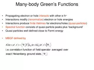
Many-body Green’s Functions. Propagating electron or hole interacts with other e - /h + Interactions modify ( renormalize ) electron or hole energies Interactions produce finite lifetimes for electrons/holes ( quasi-particles )

Many-body Green’s Functions
E N D
Presentation Transcript
Many-body Green’s Functions • Propagating electron or hole interacts with other e-/h+ • Interactions modify (renormalize) electron or hole energies • Interactions produce finite lifetimes for electrons/holes (quasi-particles) • Spectral function consists of quasi-particle peaks plus ‘background’ • Quasi-particles well defined close to Fermi energy • MBGF defined by
Add particle Remove particle t’ t > t’ time Go(x,y) y,t’ x,t Remove particle Add particle t t’ > t G(x,y) time y,t’ x,t Many-body Green’s Functions • Space-time interpretation of Green’s function • (x,y) are space-time coordinates for the endpoints of the Green’s function • Green’s function drawn as a solid, directed line from y to x • Non-interacting Green’s function Go represented by a single line • Interacting Green’s Function G represented by a double or thick single line y x x y
Many-body Green’s Functions • Lehmann Representation(F 72 M 372) physical significance of G
Many-body Green’s Functions • Lehmann Representation (physical significance of G)
Many-body Green’s Functions • Lehmann Representation (physical significance of G)
Many-body Green’s Functions • Lehmann Representation (physical significance of G) • Poles occur at exact N+1 and N-1 particle energies • Ionisation potentials and electron affinities of the N particle system • Plus excitation energies of N+1 and N-1 particle systems • Connection to single-particle Green’s function
Many-body Green’s Functions • Gell-Mann and Low Theorem (F 61, 83) • Expectation value of Heisenberg operator over exact ground state expressed in terms of evolution operators and the operator in question in interaction picture and ground state of non-interacting system
Many-body Green’s Functions • Perturbative Expansion of Green’s Function (F 83) • Expansion of the numerator and denominator carried out separately • Each is evaluated using Wick’s Theorem • Denominator is a factor of the numerator • Only certain classes of (connected) contractions of the numerator survive • Overall sign of contraction determined by number of neighbour permutations • n = 0 term is just Go(x,y) • x, y are compound space and time coordinates i.e. x≡ (x, y, z, tx)
Many-body Green’s Functions • Fetter and Walecka notation for field operators (F 88)
+ + + ˆ ˆ ˆ ˆ ˆ ˆ ψ ( r ) ψ ( r ' ) ψ ( r ' ) ψ ( r ) ψ ( x ) ψ ( y ) (1) (-1)3 (i)3v(r,r’)Go(r’,r) Go(r,r’) Go(x,y) + + + (-1)4(i)3v(r,r’)Go(r,r) Go(r’,r’) Go(x,y) ˆ ˆ ˆ ˆ ˆ ˆ ψ ( r ) ψ ( r ' ) ψ ( r ' ) ψ ( r ) ψ ( x ) ψ ( y ) (2) + + + ˆ ˆ ˆ ˆ ˆ ˆ (-1)5(i)3v(r,r’)Go(x,r) Go(r’,r’) Go(r,y) ψ ( r ) ψ ( r ' ) ψ ( r ' ) ψ ( r ) ψ ( x ) ψ ( y ) (3) + + + ˆ ˆ ˆ ˆ ˆ ˆ (-1)4(i)3v(r,r’)Go(r’,r) Go(x,r’) Go(r,y) ψ ( r ) ψ ( r ' ) ψ ( r ' ) ψ ( r ) ψ ( x ) ψ ( y ) (4) + + + ˆ ˆ ˆ ˆ ˆ ˆ ψ ( r ) ψ ( r ' ) ψ ( r ' ) ψ ( r ) ψ ( x ) ψ ( y ) (5) (-1)6(i)3v(r,r’)Go(x,r) Go(r,r’) Go(r’,y) + + + ˆ ˆ ˆ ˆ ˆ ˆ ψ ( r ) ψ ( r ' ) ψ ( r ' ) ψ ( r ) ψ ( x ) ψ ( y ) (6) (-1)7(i)3v(r,r’)Go(r,r) Go(x,r’) Go(r’,y) Many-body Green’s Functions • Nonzero contractions in numerator of MBGF
x -(i)3v(r,r’)Go(r’,r) Go(r,r’) Go(x,y) (1) x r’ r +(i)3v(r,r’)Go(r,r) Go(r’,r’) Go(x,y) (2) (2) (1) r r’ y x x y -(i)3v(r,r’)Go(x,r) Go(r’,r’) Go(r,y) (3) r r’ r’ r r’ r +(i)3v(r,r’)Go(r’,r) Go(x,r’) Go(r,y) (4) y y y (3) (4) x x +(i)3v(r,r’)Go(x,r) Go(r,r’) Go(r’,y) (5) r r’ -(i)3v(r,r’)Go(r,r) Go(x,r’) Go(r’,y) (6) y (5) (6) Many-body Green’s Functions • Nonzero contractions
(-1)3(i)2v(r,r’)Go(r’,r) Go(r,r’) (-1)4(i)2v(r,r’)Go(r,r) Go(r’,r’) (8) r’ r r r’ Denominator = 1 + + + … (7) Numerator = [ 1 + + + … ] x [ + + + … ] Many-body Green’s Functions • Nonzero contractions in denominator of MBGF • Disconnected diagrams are common factor in numerator and denominator
iG(x, y) = + + + … Many-body Green’s Functions • Expansion in connected diagrams • Some diagrams differ in interchange of dummy variables • These appear m! ways so m! term cancels • Terms with simpleclosed loop contain time ordered product with equal times • These arise from contraction of Hamiltonian where adjoint operator is on left • Terms interpreted as
Many-body Green’s Functions • Rules for generating Feynman diagrams in real space and time (F 97) • (a) Draw all topologically distinct connected diagrams with m interaction lines and 2m+1 directed Green’s functions. Fermion lines run continuously from y to x or close on themselves (Fermion loops) • (b) Label each vertex with a space-time point x = (r,t) • (c) Each line represents a Green’s function, Go(x,y), running from y to x • (d) Each wavy line represents an unretarded Coulomb interaction • (e) Integrate internal variables over all space and time • (f) Overall sign determined as (-1)F where F is the number of Fermion loops • (g) Assign a factor (i)m to each mth order term • (h) Green’s functions with equal time arguments should be interpreted as G(r,r’,t,t+) where t+ is infinitesimally ahead of t • Exercise: Find the 10 second order diagrams using these rules
q2 q3 q1 Many-body Green’s Functions • Feynman diagrams in reciprocal space • For periodic systems it is convenient to work in momentum space • Choose a translationally invariant system (homogeneous electron gas) • Green’s function depends on x-y, not x,y • G(x,y) and the Coulomb potential, V, are written as Fourier transforms • 4-momentumis conserved at vertices 4-momentum Conservation Fourier Transforms
Many-body Green’s Functions • Rules for generating Feynman diagrams in reciprocal space • (a) Draw all topologically distinct connected diagrams with m interaction lines and 2m+1 directed Green’s functions. Fermion lines run continuously from y to x or close on themselves (Fermion loops) • (b) Assign a direction to each interaction • (c) Assign a directed 4-momentum to each line • (d) Conserve 4-momentum at each vertex • (e) Each interaction corresponds to a factor v(q) • (f) Integrate over the m internal 4-momenta • (g) Affix a factor (i)m/(2p)4m(-1)F • (h) A closed loop or a line that is linked by a single interaction is assigned a factor eied Go(k,e)
Equation of Motion for the Green’s Function • Equation of Motion for Field Operators (from Lecture 2)
Equation of Motion for the Green’s Function • Equation of Motion for Field Operators
Equation of Motion for the Green’s Function • Differentiate G wrt first time argument
Equation of Motion for the Green’s Function • Differentiate G wrt first time argument
x r1 x r1 (9) (10) y y Equation of Motion for the Green’s Function • Evaluate the T product using Wick’s Theorem • Lowest order terms • Diagram (9) is the Hartree-Fock exchange potential x Go(r1,y) • Diagram (10) is the Hartree potential x Go(x,y) • Diagram (9) is conventionally the first term in the self-energy • Diagram (10) is included in Ho in condensed matter physics (i)2v(x,r1)Go(x,r1) Go(r1,y) (i)2v(x,r1)Go(r1,r1) Go(x,y)
x r1 S(x,1) (i)3v(1,2) v(x,r1)Go(1,x) Go(r1,2) Go(2,r1)Go(1,y) 1 2 Go(1,y) y (11) Equation of Motion for the Green’s Function • One of the next order terms in the T product • The full expansion of the T product can be written exactly as
x x x’ (9) (10) x’ Equation of Motion for the Green’s Function • The proper self-energy S* (F 105, M 181) • The self-energy has two arguments and hence two ‘external ends’ • All other arguments are integrated out • Proper self-energy terms cannot be cut in two by cutting a single Go • First order proper self-energy terms S*(1) • Hartree-Fock exchange term Hartree (Coulomb) term Exercise: Find all proper self-energy terms at second order S*(2) r1
Equation of Motion for the Green’s Function • Equation of Motion for G and the Self Energy
Equation of Motion for the Green’s Function • Dyson’s Equation and the Self Energy
Equation of Motion for the Green’s Function • Integral Equation for the Self Energy
G(x,y) = = + + + … S(x’,x’’)= + + … Equation of Motion for the Green’s Function • Dyson’s Equation (F 106) • In general, S* is energy-dependent and non-Hermitian • Both first order terms in S are energy-independent • Quantum Chemistry: first order self energy terms included in Ho • Condensed matter physics: only ‘direct’ first order term is in Ho • Single-particle band gap in solids strongly dependent on ‘exchange’ term
a, q a+b, ℓ+q b, ℓ w-a, k-q a, q a+b, ℓ+q b, ℓ Evaluation of the Single Loop Bubble • One of the 10 second order diagrams for the self energy • The first energy dependent term in the self-energy • Evaluate for homogeneous electron gas (M 170)
y x Evaluation of the Single Loop Bubble • Polarisation bubble:frequency integral over b • Integrand has poles at b = e ℓ - id and b = -a + e ℓ+q + id • The polarisation bubble depends on q and a • There are four possibilities for ℓ and q
y x Evaluation of the Single Loop Bubble • Integral may be evaluated in either half of complex plane
Evaluation of the Single Loop Bubble • From Residue Theorem • Exercise: Obtain this result by closing the contour in the lower half plane
Evaluation of the Single Loop Bubble • Polarisation bubble: continued • For • Both poles in same half plane • Close contour in other half plane to obtain zero in each case • Exercise: For • Show that • And that
a, q a+b, ℓ+q b, ℓ w-a, k-q a, q Evaluation of the Single Loop Bubble • Self Energy
Evaluation of the Single Loop Bubble • Self Energy: continued
Evaluation of the Single Loop Bubble • Real and Imaginary Parts • Quasiparticle lifetime tdiverges as energies approach the Fermi surface