Industrial Engineering Optimization: Algorithms and Software Solutions
Learn to solve industrial engineering problems via optimization modeling, algorithms, teamwork, and software utilization. Delve into optimization algorithms, decision variables, and mathematical program analysis in this course.

Industrial Engineering Optimization: Algorithms and Software Solutions
E N D
Presentation Transcript
IE 312 Optimization Siggi Olafsson 3018 Black olafsson@iastate.edu
Optimization • In this class you will learn to solve industrial engineering problems by modeling them as optimization problems • You will understand common optimization algorithms for solving such problems • You will learn the use of software for solving complex problems, and you will work as part of a team to address complex ill-structured problems with multiple solutions
Optimization Formulation Decision variables: Integer programming problem: This is a variant of what is called the knapsack problem
How about the traveling salesman? What is the shortest route that visits each city exactly once?
The Process Problem Problem Formulation Model Analysis Conclusions
Problem Formulation • What is the objective function? • Maximize profit, • Minimize inventory, ... • What are the decision variables? • Capacity, routing, production and stock levels • What are the constraints? • Capacity is limited by capital • Production is limited by capacity
Mathematical Programs Decision variables
Analysis • Optimization Algorithm • Computer Implementation • Excel (or other spreadsheet) • Optimization software (e.g., LINDO) • Modeling software (e.g., LINGO) Increasing Complexity
Optimization Algorithms • Find an initial solution • Loop: • Look at “neighbors” of current solution • Select one of those neighbors • Decide if to move to selected solution • Check stopping criterion
In This Class You Will … • Learn problem formulation (modeling) • Learn selecting appropriate algorithms • Learn using those algorithms
Academic Honesty You are expected to be honest in all of your actions and communications in this class. Students suspected of committing academic dishonesty will be referred to the Dean of Students Office as per University policy. For more information regarding Academic Misconduct see http://www.dso.iastate.edu/ja/academic/misconduct.html
Professionalism You are expected to behave in a professional manner during this class.
The OR Process Problem (System) Problem Formulation Model Analysis Conclusions
Problem Formulation • Capture the essence of the system • Variables • Relationships • Ask ourselves: • What is the objective? • What are the decision variables? • What are the constraints?
Mortimer Middleman • Wholesale diamond business • sale price $900/carat • average order 55 carats/week • International market • purchase price $700/carat • minimum order 100 carats/trip • trip takes one week and costs $2000
Inventory Problem • Cost of keeping inventory • insurance • tied up capital • 0.5% of wholesale value/week • Cost of not keeping inventory • lost sales (no backordering)
The Current Situation • Holding cost of $38,409 in past year • Unrealized profits of $31,600 • Resupply travel cost $24,000 • Total of $94,009 • Can we do better? • How do we start answering that question?
Problem Formulation • What are the decision variables? • When should we order? • Reorder point r (quantity that trigger order) • How much should we order? • Order quantity q • Note that this grossly simplifies the reality of Mortimer’s life!
Problem Formulation • What are the constraints? • What is the objective? • Minimize cost • Holding cost • Replenishment cost • Lost-sales cost
Relationships(System Dynamics) • Assumptions • Constant-rate demand • Is this a strong or weak assumption? • Is this assumption realistic?
System Dynamics With safety stock No safety stock or lost sales With lost sales r r r 1 week 1 week 1 week Why might we get lost sales despite our planning? Can we ignore this?
Assuming No Lost Sales • No lost sales implies r 55 • Cycle length • Average inventory
Optimization Model Minimize Subject to
Solving the Problem (Analysis) • Feasible solution • Any set of values that satisfies the constraints • Optimal solution • A feasible solution that has the best possible objective function value • Algorithms: • Find a feasible solution • Try to improve on it
A Solution for Mortimer • What are some feasible solutions? • The smallest feasible value of r is 55 • What happens if we change it to 56? • Increased holding cost! • ‘Clearly’ the optimal replenishment point is
New Optimization Problem Minimize Subject to Differentiate the objective function and set equal to zero:
Optimal Solution Optimum
Economic Order Quantity (EOQ) Cost of replenishment Classical result in inventory theory: Holding cost Lead time (replenishment) Weekly demand
Discussion • Sensitivity Analysis • Exploring how the results change if parameters change • Why is this important? • Closed-Form Solutions • Final result a simple formula in terms of the input variables • Very fast computationally • Makes sensitivity analysis very easy
Evaluating the Model • Tractability of Model • Ease by which we can analyze the model • Validity • The degree by which inferences drawn from model also hold for actual system • Trade-Off! • A “Good” Model is Tractable and Valid
Model Validity • A model is valid for a specific purpose • It only has to answer the questions we ask correctly! • Recipe for a Good Model • Start with a simple model • Evaluate assumptions • Does adding complexity change the outcome? • Relax assumption/add constraint
Validity of Our Model • Customer demand (average 55)
Simulation Analysis • Using the same conceptual model, we can simulate the performance using the historical data • Check if Mortimer is due with a shipment • Check if a new trip is warranted • Reduce inventory by actual demand • Simulation of our policy q=251, r=55 implies a cost of $108,621
Evaluation of Cost • Our predicted cost is • Mortimer’s current cost is $94,009 • The simulated cost is $108,621
Simulation Validity • Which model should we trust: • The simulation model that predicts a performance of $108,621, or • the EOQ model that predicts a performance of $45,630? • Examine the assumptions made: • EOQ model: constant demand • Simulation: future identical to past • In general, simulation models have a high degree of validity
Descriptive vs Prescriptive • How about tractability? • What does the simulation tell us? How easy is it to do sensitivity analysis? • Descriptive models • Only evaluate an alternative or solution • Prescriptive models • Suggest a good (or optimal) alternative
Numerical Search • We can use our descriptive simulation model to look for a better solution • Algorithm: • Start with an initial (good) solution • Check ‘similar’ solution (neighbors) • Select one of the neighbors • Repeat until a stopping criterion is satisfied
Search for Reorder Point $64,242 $63,054 $63,254 $108,421 $108,621
Search for Order Quantity $63,054 $72,781 $95,193 Best Point Found
Evaluation • We have found a solution q=251, r=85 with cost $63,054 • Better than current ($94,009) and previously obtained solution ($108,621) • Is this the best solution? • We don’t know! • What if we started with a different initial solution?
A New Search 59,539 Initial Solution 56,904 58,467 54,193 56,900 59,732 Best Point Found
Heuristic vs Optimal • Optimal Solution • Solution that is gives the best objective function value • Heuristic Solution • A ‘good’ feasible solution • Should we demand optimality? • Inaccurate search vs approximation in model
Deterministic vs Stochastic Models • Our deterministic simulation model assumed future identical to past • Not true! Demand is random • Stochastic simulation fits a random distribution to the historical data • The world is stochastic • Why not always use stochastic models? • Tractability versus validity
Mathematical Programming • Deterministic models • Assume all data known with certainty • Validity • Often produce valid results • Tractability • Easier than stochastic models • Known as mathematical programming
Problem Formulation • Decision variables • Constraints • Variable-type constraints • Main constraints • Objective function
Two Crude Petroleum $20 9000 barrels/day 2000 barrels Gasoline Saudi Arabia 1500 barrels Jet Fuel Refinery Venezuela 500 barrels Lubricants $15 6000 barrels/day
Oil Processing Data • Barrel of Saudi Crude • 0.3 barrels of gasoline • 0.4 barrels of jet fuel • 0.2 barrels of lubricant • Barrel of Venezuela Crude • 0.4 barrels of gasoline • 0.2 barrels of jet fuel • 0.3 barrels of lubricant
Decision Variables • What can we control or decide upon? • How much of each crude • Thus, define • Clearly define what you mean!
Constraints • Variable-type constraints • Domain of decision variables (most often a range) • Very simple here:

