Download
1 / 33
340 likes | 808 Vues
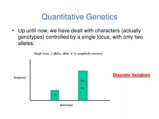
Footprints of Diversity in the Agricultural Landscape: Understanding and Creating Spatial Patterns of Diversity. Quantitative Genetics and Genetic Diversity. Bruce Walsh Depts of Ecology & Evol. Biology, Animal Science, Biostatistics, Plant Science. Overview. Introductory comments

E N D
Footprints of Diversity in the Agricultural Landscape: Understanding and Creating Spatial Patterns of Diversity Quantitative Genetics and Genetic Diversity Bruce Walsh Depts of Ecology & Evol. Biology, Animal Science, Biostatistics, Plant Science
Overview • Introductory comments • Processes generating spatial genetic variation • Molecular vs. genetic variation • Importance of different types of variability • Finding genomic locations under selection • Patterns selection leaves in the genome • Finding genes involved in local adaptation • G x E tools for localizing interesting populations • Use of factorial regressions to dissect contributions to G x E
Divergence of populations over time • The patterning of genetic variation within- and between-populations is a dynamic process • Loss/fixation of variations via drift and creation of new genetic variation via mutation (and perhaps migration) is a constant background process • Populations can also evolve via natural selection to be locally-adaptive
Populations show both within-population variation as well as between-population variation (divergence) In this example, lots of within-population variation, little between-population variation (little divergence)
Shared alleles is a private allele is a private allele Over time, loss/fixation (via drift) of variation increases the between-population variation unless overpowered by sufficient levels of migration Here, plenty of within-population variation, but also significant between-population variation as well.
Variation can also be lost (and hence between-population variation increased) in founder populations Note reduction of within-population variation relative to founding (source) population
Quantifying levels of variation • In an ANOVA-like framework, we can ask how much of the total variation over a series of population is in common (within-population variation) and how much is distinct (between-population variation), such as differences in allele frequencies • FST = fraction of all genetic variation due to between-population divergence (RST when using SSR/STR). • Range is 0 to 1 • The larger the value of FST, the more molecular divergence
Molecular diversity • SNPs, SSRs (STRs), and other molecular markers widely used to examine genetic variation within populations and divergence between them (such as estimating levels of polymorphism and FST). • Much of this pattern of variation is largely shaped by the genetic drift of effectively neutral alleles (the marker alleles) • Hence, molecular variation is a snap-shot of the neutral variation • All loci equally influenced by demography
Genetic divergence • Drift and mutation cause allele frequencies to change between populations • However, the breeder is usually interested in those genetic changes from selection: • Adaptation to the local environment • Interested in both traits that provide adaptation • and in the genes that underlie these adaptive traits
Types of divergence • Three sources of usable genetic variation for breeding from population divergence • Accumulation of new QTLs alleles for subsequent selection response • Divergence in allele frequencies at loci involved in heterosis • Fixation of locally-adaptive mutations. • How good a predictor is divergence at neutral sites (e.g., SNP, STR data) likely to be for these three classes?
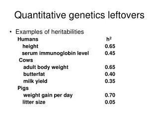
Accumulation of new variation • For random quantitative traits, new variance accumulates at roughly 2t Var(M) • The trait mutational variance/gen, Var(M), is typically on the order of 1/1000 of the environmental variance (slow, but steady) • Accumulation of variation in a neutral trait tracks the accumulation of divergence at random molecular markers • As a rough approximation, molecular divergence can provide a guide of potentially usable quantitative trait variation
Predicts that usable variance can be generated in the cross between two molecularly-divergent lines. • Stronger prediction: Larger FST, larger F2 variation in cross • Transgressive segregation is a potential example of this, the finding in many QTL mapping studies that favorable alleles for a trait are often found in populations with lower trait values (and vise-versa)
Accumulation of heterotic variation Recall that the expected heterosis in a cross between two populations is a function of their difference (dp) in allele frequencies at loci showing dominance (d) HF1 = Si (dpi)2di dp2 = variance under drift = 2p(1-p)[1-exp(-t/Ne)] Hence, dp2 is expected to increase with divergence time (t), which can be predicted by levels of molecular divergence (larger FST, greater divergence time).
Predicting heterosis • While expected allele frequency differences increase with time of divergence, this does not guarantee that heterosis will increase with divergence time between populations • Key is that strong directional dominance (d > 0 consistently) is required, and drift also increases the frequency differences in alleles with d < 0. • Hence, level of marker divergence is a poor predictor of cross heterosis. • FST a poor predictor of HF1
Finding genes under selection • Overall amount of genomic molecular divergence no predictor of potential adaptation • Can have large amounts of neutral divergence (large FST), but little to no adaptation. • Likewise, populations with small FST can have undergone considerable adaptation, esp. when strong selection has occurred • However, can use molecular markers to look for recent signatures of selection in genomic regions • This, in turn, allows us to localize potential adaptation genes
Search for Genes that experienced artificial (and natural) selection Akin in sprit to testing candidate genes for association or using genome scans to find QTLs. In linkage studies: Use molecular markers to look for marker-trait associations (phenotypes) In tests for selection, use molecular markers to look for patterns of selection (patterns of within- and between-species variation) Tests for selection make NO assumptions as to the traits under selection
Logic behind polymorphism-based tests Key: Time to MRCA relative to drift If a locus is under positive selection, more recent MRCA (shorter coalescent) If a locus is under balancing selection, older MRCA relative to drift (deeper coalescent) Shorter coalescent = lower levels of variation, longer blocks of disequilibrium Deeper coalescent = higher levels of variation, shorter blocks of disequilibrium
Time Time to MRCA for the individuals sampled Selective Sweep Past Neutral Balancing selection Present Selection changes to coalescent times Longer time back to MRCA Shorter time back to MRCA
A scan of levels of polymorphism can thus suggest sites under selection Directional selection (selective sweep) Variation Local region with reduced mutation rate Map location Balancing selection Variation Local region with elevated mutation rate Map location
Example: maize domestication gene tb1 Wang et al. (1999) observed a significant decrease in genetic variation in the 5’ NTR region of tb1, suggesting a selective sweep influenced this region. Wang et al (1999) Nature 398: 236.
Polymorphism-based tests • Given a sample of n sequences at a candidate gene, there are several different ways to measure diversity, which are related under the strict neutral model • number of segregating sites. E(S) = anq • number of singletons. E(h) = q* n/(n-1) • average num. of pairwise differences, E(k) = q • A number of polymorphism-based tests (e.g., Tajima’s D) are based on detecting departures from these expectations, e.g., E(S) differing from an E(k)
Major Complication With Polymorphism-based tests Demographic factors can also cause these departures from neutral expectations! Too many young alleles -> recent population expansion Too many old alleles -> population substructure Thus, there is a composite alternative hypothesis, so that rejection of the null does not imply selection. Rather, selection is just one option.
Can we overcome this problem? It is an important one, as only polymorphism- based tests can indicate on-going selection Solution: demographic events should leave a constant signature across the genome Essentially, all loci experience common demographic factors Genome scan approach: look at a large number of markers. These generate null distribution (most not under selection), outliers = potentially selected loci (genome wide polymorphism tests)
Linkage Disequilibrium Decay One feature of a selective sweep are derived alleles at high frequency. Under neutrality, only older alleles are at higher frequencies. Such a feature is NOT influenced by past demography. Older = more time to reduce the size of LD (haplotype) blocks Sabeti et al (2002) note that under a sweep such high frequency young alleles should (because of their recent age) have much longer regions of LD than expected. Wang et al (2006) proposed a Linkage Disequilibrium Decay, or LDD, test looks for excessive LD for high frequency alleles
Starting haplotype Under directional selection, very fast change in allele frequency, and hence short time. Results in high-frequency alleles with long haplotypes freq Under pure drift, high-freq alleles should have short haplotypes time
Optimal conditions for detecting selection High levels of polymorphism at the start of selection High effective levels of recombination gives a shorter window around the selective site Low selfing as high levels of selfing reduces the effective recombination rate Recent selection, as signatures of sweeps persist for roughly Ne generations
Summary: Detecting Adaptive Genes Linkage mapping (QTL mapping, association analysis) vs. detection of selected loci Linkage: Know the target phenotype(s) Selection: Don’t know the target phenotype Both can suffer from low power and confounding from demographic effects Both can significantly benefit from high-density genomic scans, but these are also not without problems.
G x E • The flip side of molecular divergence is the direct assessment of trait values in a set of populations/lines over a series of environments • Lines that show strong positive G x E (genotype-environment interactions) in a particular environment (or set of environments) are sources of improvement genes for a target environment(s)
Basic G x E model • Basic model is the mean value of line i in environment j is u + Gi + Ej + GEij • Giis the line average over all environments • Ej is the environmental effect over all lines • GEij is the G x E interaction
Looking for structure in G x E • Often there is considerable structure in G x E, so that the ij-th term can be estimated as a simple product • GEij = aibj • General bilinear models can be used (more terms) • Key: ai can be thought of an a genotypic environmental specificity factor • Modification is to use factorial regression • Here one uses measured environmental factors (temp, rainfall, etc) to try to predict GE • One can also incorporate measured genes (candidate genotypes entered as cofactors) as well
GEij = h1iy1j + … hpi ypj + dij • Suppose that y1 .. yp are p environmental factors that are measured by the breeder (e.g., degree days, rainfall,etc.), with ykj the value of factor k in environment j • The idea is to predict GE by looking at how different lines react to each environmental factor • h1i is the measure of the sensitivity to line i to environmental factor 1, h2i to factor 2, etc.
Factorial regressions allow the breeder to examine how each line reacts to a variety of environmental factors, potentially offering differential targets of selection • Maize example (Epinat-Le Signor et al. 2001) • A major contributor to GxE was the interaction between a line's date of flowering and water supply, with early varieties becoming more favorable as the water supply decreases
Summary • Level of genome-wide divergence using molecular markers • a weak signal for usable QTL variation • a very poor (at best!) signal for heterosis • No signal for presence of locally-adaptive genes • Signals of adaptive genes • Changes in polymorphism levels around target • Use of factorial regressions to tease out components of GXE • Environmental factors within E • Traits, genes within lines