1 / 48

Figure 6.1 Histogram of temperature data.

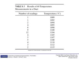
Figure 6.1 Histogram of temperature data. Figure 6.2 Some shapes of distributions: (a) symmetric; (b) skewed; (c) J-shaped; (d) bimodal; (e) uniform. (After Johnson, 1988.). Figure 6.3 Relative frequencies of duct temperatures. Figure E6.1. Figure E6.2.

Télécharger la présentation

Figure 6.1 Histogram of temperature data.

An Image/Link below is provided (as is) to download presentation Download Policy: Content on the Website is provided to you AS IS for your information and personal use and may not be sold / licensed / shared on other websites without getting consent from its author. Content is provided to you AS IS for your information and personal use only. Download presentation by click this link. While downloading, if for some reason you are not able to download a presentation, the publisher may have deleted the file from their server. During download, if you can't get a presentation, the file might be deleted by the publisher.

E N D

Presentation Transcript


  1. Figure 6.1 Histogram of temperature data.

  2. Figure 6.2 Some shapes of distributions: (a) symmetric; (b) skewed; (c) J-shaped; (d) bimodal; (e) uniform. (After Johnson, 1988.)

  3. Figure 6.3 Relative frequencies of duct temperatures.

  4. Figure E6.1

  5. Figure E6.2

  6. Figure 6.4 Normal distribution function.

  7. Figure 6.5 Standard normal distribution function.

  8. Table 6.3 (continued) Area Under the Normal Distribution From z = 0 to z

  9. Table 6.3 (continued) Area Under the Normal Distribution From z = 0 to z

  10. Table 6.3 (continued) Area Under the Normal Distribution From z = 0 to z

  11. Figure E6.9a,b

  12. Figure E6.9c,d

  13. Figure 6.6 Distribution suitable for lognormal analysis.

  14. Figure 6.7 Concept of confidence interval of the mean.

  15. Figure 6.8 Probability density function using the Student’s t-distribution.

  16. Figure 6.9 Confidence interval for the t-distribution.

  17. Table 6.6 (continued) Student's t as a function of  and

  18. Figure 6.10 Chi-squared distribution function.

  19. Figure 6.11 Confidence interval for the chi-squared distribution.

  20. Table 6.7 (continued) Critical Values of the Chi-Squared Distribution

  21. Table 6.7 (continued) Critical Values of the Chi-Squared Distribution

  22. Figure 6.12 Data showing variation in scatter of the dependent variable, y.

  23. Table 6.9 (continued) Minimum Values of the Correlation Coefficient for Significance Level 

  24. Figure E6.19

  25. Figure 6.13 Fitting a straight line through data.

  26. Figure 6.14 Least-squares line with forced origin.

  27. Figure E6.20

  28. Figure 6.15 x–y data showing an outlier.

  29. Figure 6.16 Plot of standardized residuals.

  30. Figure 6.17 Nonlinear data.

  31. Figure 6.18 Normalized residuals for nonlinear data.

  32. Figure E6.23a

  33. Figure E6.23b

  34. Figure E6.24a

  35. FigureE6.24b

  36. Figure E6.26 Caption

  37. Figure E6.27 Caption

  38. Figure P6.81

More Related