
Image Transformations through Matrices
E N D
Presentation Transcript
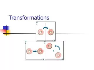
Transformations • We want to be able to make changes to the image • larger/smaller • rotate • move • This can be efficiently achieved through mathematical operations known as transformations
Transformations • We will transform the endpoints only • If we then draw the (new) lines between the transformed endpoints, we get the transformed image • This only works for certain types of transformations known as affine transformations • Such transformations preserve lines and distances and relative proportions • i.e., points on the same line before remain on the same line after an affine transformation
Transformations • Three transformations that fall into this category are • Scaling • Rotation • Translation
But First… • We’re going to need a bit of math… • … just enough to get the general idea
Matrices • Matrix • 2 dimensional array (of numbers) • m x n matrix • m rows • n columns
Matrices • Matrix • 2 dimensional array (of numbers) • m x n matrix • m rows • n columns • xij is the entry at row I, column j 2 rows 3 columns
Some Examples • a 2 x 1 matrix • A 3 x 3 matrix • 1 x 2 matrix • 2 x 2 matrix
Matrix Multiplication • In matrix multiplication, elements in the result matrix are obtained by taking the sums of the products of the elements of a row of the first with a column of the second • Calculating the sum of products of the ith row with the jth column produces the element at location [i][j]
Matrix Multiplication • In order to calculate a sum of products, the length of a row of the first matrix must be equal to the length of a column in the second matrix • length of a row = # columns • length of a column = # rows 3 columns row column 3 rows
Matrix Multiplication • Can therefore only multiply m x k matrix with a k x n matrix • # of columns of first operand = # rows of second operand • Results in an m x n matrix 3 rows 3 rows 2 rows 4 columns 2 columns 4 columns
An Example (1 1) + (2 5) = 1 + 10 = 11
An Example (1 2) + (2 6) = 2 + 12 = 14
An Example (1 3) + (2 7) = 3 + 14 = 17
An Example (1 4) + (2 8) = 4 + 16 = 20
An Example (3 1) + (4 5) = 3 + 20 = 23
An Example (3 2) + (4 6) = 6 + 24 = 30
An Example (3 3) + (4 7) = 9 + 28 = 37
An Example (3 4) + (4 8) = 12 + 32 = 44
An Example (5 1) + (6 5) = 5 + 30 = 35
An Example (5 2) + (6 6) = 10 + 36 = 46
An Example (5 3) + (6 7) = 15 + 42 = 57
An Example (5 4) + (6 8) = 20 + 48 = 68
The Algorithm multiply(a, b) // a = M x K b = K x N result = new Matrix(m, n) for i = 1, M // M rows in a for j = 1, N // N columns in b result[i][j] = 0 for k = 1, K // K columns in a, rows in b result[i][j] += a[i, k] * b[k, j] return result
What’s this got to do with us? • Matrices are a convenient and powerful way of expressing transformations • Allows complex sequences of complex transformations to be easily expressed and calculated • Let’s look at one simple transformation and see how
Scaling • Transformation that enlarges or reduces image
Scaling • Scaling can be done in the x-coordinate …
Scaling • … in the y-coordinate …
Scaling • … or in both …
Scaling • We could simply say that • To scale in the x-coordinate, multiply by the scaling factor • that is, to scale to double the size in the x-coordinate, simply multiply the x-coordinate of all endpoints by 2 • Similarly to reduce the size • Similarly in the y-direction
Simple enough • The above works and is totally adequate to scale • Why complicate matters? • Why even consider doing anything else?
Multiple Transformations • Will want to • scale and rotate • translate, rotate and translate again • etc,… • Don’t want to have to apply each transformation individually
Using Matrices • Let’s represent a point as a 1 x 2 matrix • We often call a 1 x n matrix a vector • Let’s reexamine multiplying this vector with a 2 x 2 matrix
Applying Matrix Multiplication • We can think of the above multiplication taking the point (x, y) and producing a new point (x', y') where • x' = ax + cy • y' = bx + dy
Transformation Matrix • We see that when a 2 x 2 matrix • is multiplied with a 1 x 2 vector representing a point … • … a new 1 x 2 vector is produced … • … that can be though of as representing a new point • We thus call the 2 x 2 matrix a transformation matrix • The matrix when applied to the original point transforms it into the new point
Where Matrix Multiplication Comes In • Looking at the above we can get a sense of how the 2 x 2 matrix transforms the point: y' x' b: the effect of the original x-value on the new y-value a: the effect of the original x-value on the new x-value d: the effect of the original y-value on the new y-value c: the effect of the original y-value on the new x-value
An Trivial Example • Following this line of thought, the matrix: b: the original x-value has no effect on the new y-value a: the original x-value has an identity effect on the new x-value d: the original y-value has an identity effect on the new y-value c: the original y-value has no effect on new x-value should transform the original point back to itself
A Trivial Example • To see that this is so: • The matrix • is called the identity matrix
Applying this to Scaling • Using this approach, let’s try to produce some transformation matrices for scaling • Let’s first scale the x-coordinate alone • We’d like • the new (transformed) x-value • to be a factor of the original x-value • not be affected by the original y-value • the new (transformed) y-value • to be identical to the original x-value • (not be affected by the original x-value)
Doubling the Size in the x-Direction • As an example, to double the x-value • We’d like • the new (transformed) x-value • to be 2 times the original x-value • not be affected by the original y-value • the new (transformed) y-value • to be identical to the original x-value • (not be affected by the original x-value)
The Effect of the Transformation Matrix • By recalling how the transformation matrix affects the original point, we can come up with the following ‘educated’ guess b: the effect of the original x-value on the new y-value a: the effect of the original x-value on the new x-value d: the effect of the original y-value on the new y-value c: the effect of the original y-value on the new x-value
Checking Our Guess • So we see indeed, our hunch was correct! • Doing the multiplication produces
Other Scaling Matrices • The same line of reasoning produces • The general transformation matrix for scaling in the x-direction alone • The general transformation matrix for scaling in the y-direction alone • The general transformation matrix for scaling in both directions For practice, verify these by doing the matrix multiplications!!
Applying Multiple Transformations • If we multiply the ‘scale x’ matrix and the ‘scale y’ matrix, we obtain the scale matrix for both
Applying Multiple Transformations • Similarly, if we multiply the ‘double size’ matrix and the ‘half size’ matrix, we obtain the identity matrix
Applying Multiple Transformations • Although we won’t prove it, it can be shown that multiplying two transformation matrices produces a transformation matrix whose effect is the first transformation followed by the second! • This result extends to three or more as well
Applying Multiple Transformations • This is a valuable result because it means we can achieve the effect of several transformation by applying a single matrix to our image rather than having to perform a sequence of transforms.
Rotations About the Origin • The next transformation involves rotating the endpoints (and therefore the line) about the point (0, 0)
Rotations About the Origin • Again, we will try to derive the transformation matrix • This one is a bit more involved and requires some trigonometry and geometry