Climate Models
Climate Models. Primary Source: IPCC WG-I Chapter 8 - Climate Models and Their Evaluation. Part 1: Model Structure. The Climate System. How do we simulate this?. Starting Point: Fundamental Laws of Physics. 1. Conservation of Mass. But - these are complex differential equations!


Climate Models
E N D
Presentation Transcript
Climate Models Primary Source: IPCC WG-I Chapter 8 - Climate Models and Their Evaluation
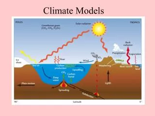
The Climate System How do we simulate this?
Starting Point: Fundamental Laws of Physics 1. Conservation of Mass But - these are complex differential equations! How can we use them? 2. First Law of Thermodynamics By solving them on a grid. 3. Newton’s Second Law Plus conservation of water vapor, chemical species, …
Global Climate Models: Structure (Bradley, 1999)
Resolution Increases over Time Computing demand increases inversely with cube of horizontal resolution. Increased computing power has allowed increased resolution
Development of Global Climate Models (GCMs) … and increasing complexity. Which should be favored?
Global Climate Models: Land-Atmosphere Link Differing scales: distributed surface properties
Global Climate Models: Development of Ocean Models (Bradley, 1999)
Global Climate Models: Parameterization Important processes smaller than a grid box: e.g., thunderstorms (atmospheric convection) few km (www.physicalgeography.net) What’s a model to do? Parameterization: Represent the effects of the unresolved processes on the grid. Assume that unresolved processes are at least partly driven by the resolved climate. (www.physicalgeography.net)
Higher Resolution Can Help Part of a Global Climate Model 2.5˚ (lat) x 3.75˚ (lon) Regional (limited-area) Climate Model ~ 0.5˚ (lat) x ~ 0.5˚ (lon)
Higher Resolution Can Help Part of a Global Climate Model 2.5˚ (lat) x 3.75˚ (lon) Regional (limited-area) Climate Model ~ 0.5˚ (lat) x ~ 0.5˚ (lon)
How Are Models Evaluated? • Testing against observations (present and past) • Comparison with other models • Metrics of reliability • Comparison with numerical weather prediction
What Limits Evaluation? • Unforced (internal) variability • Availability of Observations • Accuracy of Observations • Accuracy of Boundary Conditions (Forcing) These help determine what is “good simulation”.
GCM Simulations of Global T 58 simulations, 14 GCMs ~ 5-95% confidence limits (obs) Ensemble Average
Time Average Surface Temperature (1980-1999) ˚C Mean Model: Average of 23 GCMs
Errors in Simulated Surface Temperature (1980-1999) Lines: Observed mean Colors (top): Ensemble mean - obs. Spatial pattern correlation: ~ 98% (individual models) Colors (bottom): RMS differences in simulated-observed time series (i.e., typical error)
Annual Variability (Seasons) Lines: Observed Standard Deviation (of monthly means) Colors: Ensemble mean - observations
Diurnal Temperature Range (1980-1999) ˚C Mean Model: Average of 23 GCMs Tendency to be smaller than observed Problems with clouds? Boundary layer?
Atmospheric Zonal Average (1980-1999) K Mean Model: Average of 20 GCMs Vertical Axes: Left - Pressure (millibars) Right - Elevation (kilometers) Tendency for cool polar tropopause. Persistent feature of GCMs, though now smaller
Mean Reflected Solar Radiation (1985-1989) Average of 23 GCMs (dashed) Colors: Individual Models Satellite Observations (solid)
Mean Emitted Infrared Radiation (1985-1989) Satellite Observations (solid) Average of 23 GCMs (dashed) Colors: Individual Models
Zonal Average Precipitation (1980-1999) Observations (solid) Average of 23 GCMs (dashed) Colors: Individual Models
Annual Mean Precipitation(1980-1999) Observations Average of 23 GCMs
Atmospheric Specific Humidity (1980-1999) g/kg Mean Model: Average of 20 GCMs Vertical Axes: Left - Pressure (millibars) Right - Elevation (km) (bias) Moist bias in tropical troposphere - 40% + 40%
Ocean (Potential) Temperature (1957-1990) Mean Model: Average of 18 GCMs
Ocean Salinity (1957-1990) PSU Vertical Axes: Depth (m) Mean Model: Average of 18 GCMs PSU = “practical salinity units” • based on conductivity of electricity in water • PSU = 35 water is 3.5% salt
Ocean Heat Transport (Feb 85 - Apr 89) Models: 1980-1999
September March Sea Ice Simulation 14 GCMs (1980-1999) “Number of Models” = models with ice cover > 15% in the 2.5˚ x 2.5˚ region. Red lines: Observed 15% concentration boundaries
El Niño - Southern Oscillation (ENSO) Recent GCMs (~ 2000-2005) “Power” = amount of variability occurring for a cycle length (period) Previous generation GCMs (~ 1995-2000)
Are Models Improving? - 1 “Normalized” = RMS error / observed space-time variability
Are Models Improving? - 2 (Reichler and Kim, 2007) “Performance Index” combines error estimates of Sea level pressure Temperature Winds Humidity Precipitation Snow/Ice Ocean salinity Heat flux
Positive Feedback: Example How does Earth’s temperature get established and maintained?
Greenhouse Effect - 1 IR radiation absorbed & re-emitted, partially toward surface Solar radiation penetrates
Greenhouse Effect - 2 IR radiation absorbed & re-emitted, partially toward surface Net IR: ~25-100 W-m Emitted IR: ~200-500 W-m
Greenhouse Effect - 3 Cooler atmosphere: - Less water vapor - Less IR radiation absorbed & re-emitted Solar radiation penetrates
Greenhouse Effect - 4 Cooler atmosphere: - thus less surface warming - cooler surface temperature Solar radiation penetrates
Positive Feedback Perturb climate system Positive feedback moves climate away from starting point A destabilizing factor Other examples: - ice-albedo feedback - CO2-ocean temperature feedback
Negative Feedback Perturb climate system Negative feedback moves climate back toward starting point A stabilizing factor Example: Decrease Earth’s temperature Cooler Earth emits less radiation (energy) Outgoing radiation < solar input Net positive energy input Earth warms up from net energy input
Key Feedbacks - 1 • Water Vapor: • Warmer atmosphere can contain more water vapor • Increased water vapor increases greenhouse effect • Atmosphere warms further 2. Clouds: • Clouds cool the climate (reflect sunlight) and warm the climate (block outgoing infrared radiation) • Changes in cloud distribution can thus amplify or reduce the warming
Key Feedbacks - 2 • Snow-ice albedo: • Warmer climate has reduced snow and ice • Surface reflects less and absorbs more solar radiation • Climate warms further 2. Lapse rate (decrease of T with height): • In warmer climate, especially tropics, temperature decreases less with height • Upper troposphere warms more than surface • Upper troposphere emits energy to space (infrared radiation) more effectively than surface, countering the greenhouse effect.
END Climate Models