Climate Downscaling Using Regional Climate Models
480 likes | 765 Vues
Climate Downscaling Using Regional Climate Models. Liqiang Sun. Regional Climate Modeling. Advance our understanding of physical processes at smaller spatial and temporal scales

Climate Downscaling Using Regional Climate Models
E N D
Presentation Transcript
Climate Downscaling Using Regional Climate Models Liqiang Sun
Regional Climate Modeling • Advance our understanding of physical processes at smaller spatial and temporal scales • Advance our understanding of interactions between large and small scales and provide the physical evidence for statistical downscaling • Parameterization testbed for GCMs • Enhance the scale and relevance of climate forecast/projection • and creating information to better support decisions
Regional Climate Modeling Smaller spatial scale features developed in regional models are attributed to four types of sources: The small scale forcing, the nonlinearities presented in the atmospheric dynamical equations, hydrodynamic instabilities, and the noise generated at the lateral boundaries and model errors
There is skepticism toward RCMs in the climate community due to RCMs are not sufficiently evaluated. Most RCM efforts have been mostly isolated and unorganized. RCMs are “spreading” too fast through an inexperienced user community RCM output is taken too un-critically and it is not sufficiently “checked”
Technical Issues • Nesting Strategy • Observation • Model resolution • Domain size • Spin-up • Land initialization • Update frequency of the driving data • Quality of the driving data • Horizontal and vertical interpolation errors • Physical parameterization consistence • Climate draft or systematic errors • Bias correction
Nesting Strategy Mathematically, the abrupt change of model resolution by several times at the lateral boundaries can distort wave propagation and reflection properties. This raises an important question whether nested RCMs can accurately simulate fine-scale climate features when driven by large-scale information only. • One-Way Nesting • Two-Way Nesting • Variable Resolution Global Models
Boundary zone Perturbation damping Model inner domain Freely evolved Perturbation about basic states One-Way Nesting One-way nesting strategy has been so far the most popular approach employed by RCMs. With this approach, a RCM is “driven” by low-resolution data produced by either a GCM or by analyses of observations. As the expression “one-way” suggests, no feedback is permitted from the RCM back to the driving data. Disregard the model data in the buffer zone
Observation – high density network The existence of a good observational network is crucial for validating the RCMs’ performance.
Model Resolution • The horizontal and vertical resolutions should be fine enough to capture the local climate patterns and scales of forcings of interest (e.g., Spatial characteristics of the land surface forcing) 300KM 50KM Model Topography 10KM
Model Resolution (Cont.) 2. Availability of model dynamical and physical parameterizations. All the parameterization schemes are based on a spectral gap between the scales being parameterized and those being resolved on the grid. Therefore, all the model parameterization schemes are model resolution dependent. For example, cumulus parameterization Grid Spacing (KM) 5 20 40 ______|_______|_____________|__________ explicit ??? hybrid GCMs
20km Model Resolution (Cont.) 3. The ratio of driving data versus RCM horizontal resolution is in the range of 3-8 ( for traditional one-way nesting approach). If the downscaling grid space ratio is too large, multiple nesting is sometimes used. 80km 300km
Domain Size • The area of interest is as far as possible from the lateral buffer zone. • Model domain should encompass all regions that include forcings and circulations which directly affect climate over the area of interest. • It is preferable to place the lateral boundaries over the ocean rather than land, especially not over areas of complex topography. • It is preferable not to place the lateral boundaries over the areas with strong convection. • Internal variability usually increases with domain size • Computational Limitation
Domain Size (Cont.) Forecast area Sun et al. (2005)
Spin-up • Spin-up period is the time that model takes to achieve its climate equilibrium • Spin-up time varies depending on the domain size, season, circulation strength, and surface conditions. Atmospheric component - days Land component: top layer 0.1m - weeks root zone 1.0m - months deeper soil >1.0m - years Ocean component: upper ocean 500m - tens years deep ocean >500m - hundreds years
Land Initialization • GCMs and RCMs “see” the land differently • There are no global measurements of soil wetness and soil temperature • Spin-up time varies from weeks to years for the land variables • Continuous multiyear RCM runs - Problems related to spin-up issue can be avoided, but this is not realistic for seasonal prediction. • Proposed solution - Use of the land model off-line to generate the initial conditions for the RCM land variables • DO NOT USE GCM DATA TO INITIALIZE THE REGIONAL MODEL
Land Initialization An offline land model should be used to generate the land initial conditions for the regional climate model, or use of reanalysis data for land initialization. The resolution of the reanalysis data should be the same as or similar to that of the regional climate model. The reanalysis data should be statistically corrected. 1) calculate the standard anomaly, 2) perform statistically correction 3) corrected anomaly added to the model climatology
Update frequency of the driving data • This issue has to do with the temporal resolution of the dataset used to drive the nested RCM. As a rule of thumb, the updated period should be smaller than one quarter of the ratio of the length scale of the phase speed of the meteorological phenomena that we want to get correctly in the model domain. For instance, A typical synoptic system having a horizontal size of 1000 km and a phase speed of 50 km/h would require an updating frequency of at least 5 h. Diurnal variation is important for the tropics, it would require an updating frequency of at least 6 h. 2. Increasing the updating frequency will also introduce nesting noise. The nesting frequency of 3-6 h is mostly used.
Quality of the driving data This issue has basic implications in the concept of nested RCMs because even with a perfect model and perfect nesting scheme, the quality of the driving data used is very important. In case of a GCM driving an RCM, if the GCM large-scale circulation prediction is wrong, good results cannot be expected from the RCM. In other words, “garbage in” “garbage out”.
Quality of the driving data Case Study: Rainfall Diff:1983-1971
Horizontal and vertical and temporal interpolation errors Horizontal: the grid-point spacing and the map projections are different between the RCM and the GCM. Vertical: the grid-point spacing and the coordinates are different between the RCM and GCM. Temporal: linear interpolation between the nesting period.
Schematic of vertical and temporal incremental interpolation (Yoshimura and Kanamitsu 2009)
Physical parameterization consistence • Physics adequacy – Does a regional model have adequate representation of physics processes relevant for climate application? • Physics compatibility – Should the physics schemes in the regional model be the same as those of the GCM used to drive the regional model?
Physics adequacy All the model parameterization schemes are model resolution dependent because the parameterization schemes are based on a spectral gap between the scales being parameterized and those being resolved on the grid.
Physics adequacy (cont.) • Different physics schemes The strategy underlying the use of different physics schemes in the nested model and driving models is that each set of schemes is developed and optimized for the respective model resolutions. The disadvantage of this approach is that the interpretation of differences between nested model and driving GCM results is often difficult, because these may be caused not only by the different resolution forcings, but also by the differences in the physics schemes used.
Physics compatibility • Same physics schemes The strategy underlying the use of same physics schemes in the nested model and driving models is that maximum compatibility between the models is achieved. The main disadvantage is that physics schemes developed for coarse resolution GCMs may not be adequate for high resolutions used in nested regional models.
Physical parameterization consistence (Cont.) • Some people argue that the use of different parameterizations undermines the “validity” of the nesting technique. NOT TRUE • Successful simulations have been carried out in which the nested and driving models utilized different physics schemes. • When “perfect boundary condition” experiments are carried out, in which the LBCs are provided by analysis of observations, most regional models do not utilize the physics of the global analysis models. According to the “same physics” criterion, this should yield relatively poor and even not valid results. On the contrary, multiyear experiments driven by analyses of observations generally show better performance than GCM-driven ones, mostly because of the better overall quality of the driving field. Good (bad) quality of driving fields will lead to improved(degraded) quality of a regional model experiment, regardless of the means of how these fields are obtained.
Climate drift or systematic errors Can RCMs be run for a long time without generating systematic errors or climate drifts? All of the previously issues can contribute to systematic errors in a RCM prediction.
Bias Correction Errors from • GCM driving fields – systematical, conditional, random • nesting • RCM itself
Errors from GCM driving fields Case Study: Rainfall Diff:1983-1971 Anomaly Nesting Misra and Kanamitsu (2004)
Errors from nesting • Increase the buffer zone to allow smoother transition between the large-scale and the RCM simulated fields. assimilation of driving lateral boundary data • Make the lateral boundary forcing stronger in the upper troposphere and weaker in the lower troposphere • Place the lateral boundaries over the ocean rather than land, especially not over areas of complex topography. • Not to place the lateral boundaries over the areas with strong convection.
Errors from the RCM Typical spectral distributions of the global model and the regional model • Large-Scale Nudging Chen et al. (1999)
Recommendations for Climate Downscaling Forecasts understand the basics of what climate models are, how they work, and what their limitations are. Verify the downscaling forecasts. Use multi-model ensemble approach – coordination needed Apply model output statistics to the model raw outputs Develope new products that are both relevant and predictable - require creativity to address users’ needs
Diagnosis of Model Outputs All the variables are dynamically consistent. The RCM is a good tool for climate process studies. Examine the added values by downscaling Improvement of Spatial Patterns and Temporal Distribution Predictability at Smaller Spatial and Temporal Scales Representation of Climate Uncertainty
✗ ✔ ✗ ✗ ✔ ✗ ✗ ✔ ✔
60 km 90 km 120 km 180 km 240 km 360 km Simulation of annual mean precipitation by different resolutions of the model (mm)
A Typical Tropical Cyclone Simulated by Climate Models RSM (50km) ECHAM4.5 AGCM(T42) Vorticity Winds Vorticity Winds Precipitation Humidity Precipitation Humidity Carmago, Li and Sun (2007)
Varibility at smaller spatial and temporal scales • Diagnosis of the added benefit of dynamical downscaling • Is the local information skillful? • Is the temporal character improved?
Observation: Dec(0)-Feb(1) Qian et al. (2006)
Predictability of “weather within the climate” At seasonal lead times, there is no usable skill in forecasting on which day a locality will have precipitation, storms, temperature extremes, frontal passages, and so forth. However, there is nonetheless some skill in predicting weather statistics in the season.