Download
1 / 25
250 likes | 481 Vues
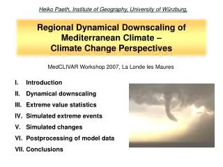
Heiko Paeth, Institute of Geography, University of Würzburg,. Regional Dynamical Downscaling of Mediterranean Climate – Climate Change Perspectives. MedCLIVAR Workshop 2007, La Londe les Maures. Introduction Dynamical downscaling Extreme value statistics Simulated extreme events

E N D
Heiko Paeth, Institute of Geography, University of Würzburg, Regional Dynamical Downscaling ofMediterranean Climate –Climate Change Perspectives MedCLIVAR Workshop 2007, La Londe les Maures • Introduction • Dynamical downscaling • Extreme value statistics • Simulated extreme events • Simulated changes • Postprocessing of model data • Conclusions
I. Introduction industrial emissions heat stress traffic emissions flood biomass burning drought over- grazing wind extremes
I. Introduction How can we infer future changes in the frequency and intensity of extreme events? • dynamical aspect (climate modelling) • statististical aspect (assessment of uncertainty)
II. Dynamical downscaling • low latitudes are dominated by convective rain events • the spatial heterogeneity of individual rain events is high • regional rainfall estimates are subject to large sampling errors
II. Dynamical downscaling station data global model regional model statist. interpol. day-to-day variability annual precipitation • station data are often too sparse to represent regional rainfall • global models are too coarse-grid for regional details • statistically interpolated data sets fail in mountainous areas • dynamic nonlinear regional models account for the effect of orography
II. Dynamical downscaling 3 x CO2 • the rainfall trends predicted by the global model are barely relevant to political plannings and measures • the rainfall trends predicted by the regional model are much more detailed and of higher amplitude • more detailed fingerprint or spatial noise added value ???
II. Dynamical downscaling Temperature differences between ensemble members at certain time scales measure of internal variability different initial conditions (stochastic) statistical comparison Precipitation variance of the ensemble mean measure of external variability • consideration of various ensemble members enables the statistical quantification of the human impact on climate in the climate model
II. Dynamical downscaling ECHAM5/MPI-OM: 2001-2050 A1B (GHG) constant LC Land degradation: 2001-2050 FAO original REMO: 2001-2050 A1B (GHG+LC) ECHAM5/MPI-OM: 1960-2000 observed GHG constant LC REMO: 1960-2000 observed GHG constant LC REMO: 2001-2050 B1 (GHG+LC) ECHAM5/MPI-OM: 2001-2050 B1 (GHG) constant LC Land degradation: 2001-2050 FAO reduced • dynamics: hydrostatic • physics: ECHAM4 • sector: 30°W-60°E ; 15°S-45°N • resolution: 0,5° ; 20 hybrid levels • validation: good results
II. Dynamical downscaling • The main features of Mediterranean climate are well reproduced by REMO.
III. Extreme value statistics f climate parameter • The processes, which cause climate extremes, are not necessarily the same as for weak climate variations. • Hence, they usually do not obey a normally distributed random process.
The Generalized Pareto Distribution (GPD) is a useful statistical distribution, since it is a parent distribution for other extreme value distributions (Gumbel, Exponential, Pareto). • The quantile function x(F) is given by: = location parameter (expectation) = scale parameter (dispersion) = shape parameter (skewness) • The parameters of the GPD can be estimated by the method of L-moments. • Estimation of T-year return values (RVs): III. Extreme value statistics cumulative GPDs dispersion parameter: threshold quantile
uncertainty of the RV estimate is inferred from bootstrap sampling: III. Extreme value statistics • from fitted GPD b random samples of size N generated • from random samples b indi- vidual RVs estimated • these b RVs are normal distri-buted such that STD is a mea-sure of the standard error of the RV estimate • signal-to-noise ratio is given by MEAN/STD over b RVs 1 cGPD N random numbers 0 mm new samples of size N f STD 90% conf. interv. RV • change in RV is significant at the 1% level, if 90% confidence inter-vals of two PDFs of RVs over b bootstrap samples do not overlap: f present-day climate forced climate RV
100-year RV in mm III. Extreme value statistics • The 100-year RV estimate ranges between 200 mm and 800 mm, depending on the random sample.
III. Extreme value statistics single estimate / simulation one predicted value without uncertainty range: pretended precision RV 2000 2050 99% probabilistic forecast with mean and uncertainty range: more objective basis for decision makers Monte Carlo approach 90% s+=84% security costs x=50% RV s-=16% 10% 2000 2050 1% • probabilistic forecast of future rainfall changes provides a reasonable scientific basis for political plannings and measures
1-year return values of heavy daily rainfall IV. Simulated extreme events • The occurrence of extreme rain events is a function of the land-sea contrast, orography, geographical latitude and seasonal cycle.
1-year return values of high daily temperature IV. Simulated extreme events • The occurrence of high temperature is also a function of the land-sea contrast, orography, geographical latitude and seasonal cycle.
IV. Simulated extreme events S/N ratio for 1-year RVs of heavy daily rainfall • The estimate of extrem values is more robust in regions and seasons with large-scale rather than convective precipitation. • The choice of long return times in the pre-sence of short time series is unappropriate.
V. Simulated changes PRECIPITATION 2025 minus present-day extremes (1y-RV) α = 5% seasonal means
V. Simulated changes TEMPERATURE 2025 minus present-day extremes (1y-RV) α = 5% seasonal means
VI. Postprocessing of model data assessed variability discontinuity daily precipitation 1840 1860 1880 1900 1920 1940 1960 1980 2000 • The assessment of changes in weather extremes is very sensitive to inhomogeneities in observational data. • No problem with model data.
VI. Postprocessing of model data different initial conditions (stochastic) radiation budget and energy fluxes atmospheric and oceanic circulation instability and convection cloud micro- physics precipitation error nonlinear error growth time • precipitation is the end product of a complex causal chain • each step imposes addititional uncertainty, particularly if it is based on a physical parameterization in the model
VI. Postprocessing of model data observed station time series (local information) REMO grid box (50km x 50km) observations: local station data climate models: area-mean precipitation comparison ? model data station data
VI. Postprocessing of model data Weather Generator simulated grid-box precipitation (dynamical part) local topography (physical part) random distribution in space (stochastical part) virtual station rainfall (result)
VI. Postprocessing of model data • REMO rainfall: - wrong seasonal cycle - underestimated extremes - hardly any dry spells • Weather Generator: - statistical distribution as observed - individual events not in phase with observations original REMO rainfall rainfall from weather generator station time series model data station data model data postprocessed
Regional climate models are required in order to account for the spatial heterogeneity of Mediterranean climate. • The estimate of extreme values and their changes requires appropriate statistical distributions and a probabilistic approach. • When estimating EVs from short time series, it is necessary to restrict the analysis to short return periods. • The occurrence of climate extremes is a function of land-sea contrast, orography, geographical latitude and seasonal cycle. • REMO projects no coherent changes in heavy rainfall whereas warm temperature extremes clearly tend to increase. • Systematic model deficiencies and the grid-box problem can be overcome by use of a weather generator. • The model results now need to be corroborated by available homogeneized long-term observational time series. VII. Conclusions