Query Optimization
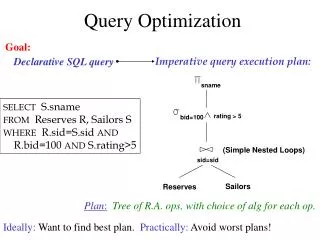
Query Optimization. Query Optimization Process (simplified a bit). Parse the SQL query into a logical tree: identify distinct blocks (corresponding to nested sub-queries or views). Query rewrite phase: apply algebraic transformations to yield a cheaper plan.

Query Optimization
E N D
Presentation Transcript
Query Optimization Process(simplified a bit) • Parse the SQL query into a logical tree: • identify distinct blocks (corresponding to nested sub-queries or views). • Query rewrite phase: • apply algebraic transformations to yield a cheaper plan. • Merge blocks and move predicates between blocks. • Optimize each block: join ordering. • Complete the optimization: select scheduling (pipelining strategy).
Operations (revisited) • Scan ([index], table, predicate): • Either index scan or table scan. • Try to push down sargable predicates. • Selection (filter) • Projection (always need to go to the data?) • Joins: nested loop (indexed), sort-merge, hash, outer join. • Grouping and aggregation (usually the last).
Algebraic Laws • Commutative and Associative Laws • R U S = S U R, R U (S U T) = (R U S) U T • R ∩ S = S ∩ R, R ∩ (S ∩ T) = (R ∩ S) ∩ T • R S = S R, R (S T) = (R S) T • Distributive Laws • R (S U T) = (R S) U (R T)
Algebraic Laws • Laws involving selection: • sC AND C’(R) = sC(sC’(R)) = sC(R) ∩ sC’(R) • sC OR C’(R) = sC(R) U sC’(R) • sC (R S) = sC (R) S • When C involves only attributes of R • sC (R – S) = sC (R) – S • sC (R U S) = sC (R) U sC (S) • sC (R ∩ S) = sC (R) ∩ S
D=E D=E Algebraic Laws • Example: R(A, B, C, D), S(E, F, G) • sF=3 (R S) = ? • sA=5 AND G=9 (R S) = ?
Algebraic Laws • Laws involving projections • PM(R S) = PN(PP(R) PQ(S)) • Where N, P, Q are appropriate subsets of attributes of M • PM(PN(R)) = PM∩N(R) • Example R(A,B,C,D), S(E, F, G) • PA,B,G(R S) = P ? (P?(R) P?(S)) D=E D=E
Query Rewrites: Sub-queries SELECT Emp.Name FROM Emp WHERE Emp.Age < 30 AND Emp.Dept# IN (SELECT Dept.Dept# FROM Dept WHERE Dept.Loc = “Seattle” AND Emp.Emp#=Dept.Mgr)
The Un-Nested Query SELECT Emp.Name FROM Emp, Dept WHERE Emp.Age < 30 AND Emp.Dept#=Dept.Dept# AND Dept.Loc = “Seattle” AND Emp.Emp#=Dept.Mgr
Converting Nested Queries Selectdistinct x.name, x.maker From product x Where x.color= “blue” AND x.price >= ALL (Select y.price From product y Where x.maker = y.maker AND y.color=“blue”)
Converting Nested Queries Let’s compute the complement first: Selectdistinct x.name, x.maker From product x Where x.color= “blue” AND x.price < SOME (Select y.price From product y Where x.maker = y.maker AND y.color=“blue”)
Converting Nested Queries This one becomes a SFW query: Select distinct x.name, x.maker From product x, product y Where x.color= “blue” AND x.maker = y.maker AND y.color=“blue” AND x.price < y.price This returns exactly the products we DON’T want, so…
Converting Nested Queries (Select x.name, x.maker From product x Where x.color = “blue”) EXCEPT (Select x.name, x.maker From product x, product y Where x.color= “blue” AND x.maker = y.maker AND y.color=“blue” AND x.price < y.price)
Semi-Joins, Magic Sets • You can’t always un-nest sub-queries (it’s tricky). • But you can often use a semi-join to reduce the computation cost of the inner query. • A magic set is a superset of the possible bindings in the result of the sub-query. • Also called “sideways information passing”. • Great idea; reinvented every few years on a regular basis.
Rewrites: Magic Sets Create View DepAvgSal AS (Select E.did, Avg(E.sal) as avgsal From Emp E Group By E.did) Select E.eid, E.sal From Emp E, Dept D, DepAvgSal V Where E.did=D.did AND D.did=V.did And E.age < 30 and D.budget > 100k And E.sal > V.avgsal
Rewrites: SIPs Select E.eid, E.sal From Emp E, Dept D, DepAvgSal V Where E.did=D.did AND D.did=V.did And E.age < 30 and D.budget > 100k And E.sal > V.avgsal • DepAvgsal needs to be evaluated only for departments where V.did IN Select E.did From Emp E, Dept D Where E.did=D.did And E.age < 30 and D.budget > 100K
Supporting Views 1. Create View PartialResult as (Select E.eid, E.sal, E.did From Emp E, Dept D Where E.did=D.did And E.age < 30 and D.budget > 100K) • Create View Filter AS Select DISTINCT P.did FROM PartialResult P. • Create View LimitedAvgSal as (Select F.did Avg(E.Sal) as avgSal From Emp E, Filter F Where E.did=F.did Group By F.did)
And Finally… Transformed query: Select P.eid, P.sal From PartialResult P, LimitedAvgSal V Where P.did=V.did And P.sal > V.avgsal
Rewrites: Group By and Join • Schema: • Product (pid, unitprice,…) • Sales(tid, date, store, pid, units) • Trees: Join groupBy(pid) Sum(units) groupBy(pid) Sum(units) Join Products Filter (price>100) Products Filter (price>100) Scan(Sales) Filter(date in Q2,2000) Scan(Sales) Filter(date in Q2,2000)
Schema for Some Examples Sailors (sid: integer, sname: string, rating: integer, age: real) Reserves (sid: integer, bid: integer, day: dates, rname: string) • Reserves: • Each tuple is 40 bytes long, 100 tuples per page, 1000 pages • Sailors: • Each tuple is 50 bytes long, 80 tuples per page, 500 pages
Query Rewriting: Predicate Pushdown Psname Psname σbid=100 AND rating >5 (Scan; write to temp T1) (Scan; write to temp T2) sid=sid σbid=100 σrating > 5 sid=sid Reserves Sailors Reserves Sailors The earlier we process selections, less tuples we need to manipulate higher up in the tree. Disadvantages?
Query Rewrites: Predicate Pushdown (through grouping) Select bid, Max(age) From Reserves R, Sailors S Where R.sid=S.sid GroupBy bid Having Max(age) > 40 Select bid, Max(age) From Reserves R, Sailors S Where R.sid=S.sid and S.age > 40 GroupBy bid • For each boat, find the maximal age of sailors who’ve reserved it. • Advantage: the size of the join will be smaller. • Requires transformation rules specific to the grouping/aggregation • operators. • Will it work work if we replace Max by Min?
Query Rewrite:Predicate Movearound Sailing wiz dates: when did the youngest of each sailor level rent boats? Select sid, date From V1, V2 Where V1.rating = V2.rating and V1.age = V2.age Create View V1 AS Select rating, Min(age) From Sailors S Where S.age < 20 Group By rating Create View V2 AS Select sid, rating, age, date From Sailors S, Reserves R Where R.sid=S.sid
Query Rewrite: Predicate Movearound Sailing wiz dates: when did the youngest of each sailor level rent boats? Select sid, date From V1, V2 Where V1.rating = V2.rating and V1.age = V2.age and age < 20 First, move predicates up the tree. Create View V1 AS Select rating, Min(age) From Sailors S Where S.age < 20 Group By rating Create View V2 AS Select sid, rating, age, date From Sailors S, Reserves R Where R.sid=S.sid
Query Rewrite: Predicate Movearound Sailing wiz dates: when did the youngest of each sailor level rent boats? Select sid, date From V1, V2 Where V1.rating = V2.rating and V1.age = V2.age and age < 20 First, move predicates up the tree. Then, move them down. Create View V1 AS Select rating, Min(age) From Sailors S Where S.age < 20 Group By rating Create View V2 AS Select sid, rating, age, date From Sailors S, Reserves R Where R.sid=S.sid, and S.age < 20.
Query Rewrite Summary • The optimizer can use any semantically correct rule to transform one query to another. • Rules try to: • move constraints between blocks (because each will be optimized separately) • Unnest blocks • Especially important in decision support applications where queries are very complex. • In a few minutes of thought, you’ll come up with your own rewrite. Some query, somewhere, will benefit from it. • Theorems?
Cost Estimation • For each plan considered, must estimate cost: • Must estimate costof each operation in plan tree. • Depends on input cardinalities. • Must estimate size of result for each operation in tree! • Use information about the input relations. • For selections and joins, assume independence of predicates. • We’ll discuss the System R cost estimation approach. • Very inexact, but works ok in practice. • More sophisticated techniques known now.
Statistics and Catalogs • Need information about the relations and indexes involved. Catalogstypically contain at least: • # tuples (NTuples) and # pages (NPages) for each relation. • # distinct key values (NKeys) and NPages for each index. • Index height, low/high key values (Low/High) for each tree index. • Catalogs updated periodically. • Updating whenever data changes is too expensive; lots of approximation anyway, so slight inconsistency ok. • More detailed information (e.g., histograms of the values in some field) are sometimes stored.
Size Estimation and Reduction Factors SELECT attribute list FROM relation list WHEREterm1AND ... ANDtermk • Consider a query block: • Maximum # tuples in result is the product of the cardinalities of relations in the FROM clause. • Reduction factor (RF) associated with eachtermreflects the impact of the term in reducing result size. Resultcardinality = Max # tuples * product of all RF’s. • Implicit assumption that terms are independent! • Term col=value has RF 1/NKeys(I), given index I on col • Term col1=col2 has RF 1/MAX(NKeys(I1), NKeys(I2)) • Term col>value has RF (High(I)-value)/(High(I)-Low(I))
Histograms • Key to obtaining good cost and size estimates. • Come in several flavors: • Equi-depth • Equi-width • Which is better? • Compressed histograms: special treatment of frequent values.
Histograms • Statistics on data maintained by the RDBMS • Makes size estimation much more accurate (hence, cost estimations are more accurate)
Histograms Employee(ssn, name, salary, phone) • Maintain a histogram on salary: • T(Employee) = 25000, but now we know the distribution
Salary Histograms Ranks(rankName, salary) • Estimate the size of Employee Ranks
Salary Histograms • Assume: • V(Employee, Salary) = 200 • V(Ranks, Salary) = 250 • Then T(Employee Ranks) = = Si=1,6 Ti Ti’ / 250 = (200x8 + 800x20 + 5000x40 + 12000x80 + 6500x100 + 500x2)/250 = ….
Plans for Single-Relation Queries(Prep for Join ordering) • Task: create a query execution plan for a single Select-project-group-by block. • Key idea: consider each possible access path to the relevant tuples of the relation. Choose the cheapest one. • The different operations are essentially carried out together (e.g., if an index is used for a selection, projection is done for each retrieved tuple, and the resulting tuples are pipelined into the aggregate computation).
SELECT S.sid FROM Sailors S WHERE S.rating=8 Example • If we have an Index on rating: • (1/NKeys(I)) * NTuples(S) = (1/10) * 40000 tuples retrieved. • Clustered index: (1/NKeys(I)) * (NPages(I)+NPages(S)) = (1/10) * (50+500) pages are retrieved (= 55). • Unclustered index: (1/NKeys(I)) * (NPages(I)+NTuples(S)) = (1/10) * (50+40000) pages are retrieved. • If we have an index on sid: • Would have to retrieve all tuples/pages. With a clustered index, the cost is 50+500. • Doing a file scan: we retrieve all file pages (500).
Determining Join Ordering • R1 R2 …. Rn • Join tree: • A join tree represents a plan. An optimizer needs to inspect many (all ?) join trees R3 R1 R2 R4
Types of Join Trees • Left deep: R4 R2 R5 R3 R1
Types of Join Trees • Bushy: R3 R2 R4 R5 R1
Types of Join Trees • Right deep: R3 R1 R5 R2 R4
Problem • Given: a query R1 R2 … Rn • Assume we have a function cost() that gives us the cost of every join tree • Find the best join tree for the query
Dynamic Programming • Idea: for each subset of {R1, …, Rn}, compute the best plan for that subset • In increasing order of set cardinality: • Step 1: for {R1}, {R2}, …, {Rn} • Step 2: for {R1,R2}, {R1,R3}, …, {Rn-1, Rn} • … • Step n: for {R1, …, Rn} • A subset of {R1, …, Rn} is also called a subquery
Dynamic Programming • For each subquery Q ⊆ {R1, …, Rn} compute the following: • Size(Q) • A best plan for Q: Plan(Q) • The cost of that plan: Cost(Q)
Dynamic Programming • Step 1: For each {Ri} do: • Size({Ri}) = B(Ri) • Plan({Ri}) = Ri • Cost({Ri}) = (cost of scanning Ri)
Dynamic Programming • Step i: For each Q ⊆ {R1, …, Rn} of cardinality i do: • Compute Size(Q) (later…) • For every pair of distinct subqueriesQ’, Q’’ s.t. Q = Q’ U Q’’compute cost(Plan(Q’) Plan(Q’’)) • Cost(Q) = the smallest such cost • Plan(Q) = the corresponding plan
Dynamic Programming • Return Plan({R1, …, Rn})


