Download

1 / 32
320 likes | 502 Vues
Nonlinear Quadratic Dynamic Matrix Control with State Estimation. Hao-Yeh Lee P rocess S ystem E ngineering Laboratory Department of Chemical Engineering National Taiwan University. Reference.

E N D
Nonlinear Quadratic Dynamic Matrix Control with State Estimation Hao-Yeh Lee Process System Engineering Laboratory Department of Chemical Engineering National Taiwan University
Reference • Gattu, G., and E. Zafiriou, “Nonlinear Quadratic Dynamic Matrix Control with State Estimation,” Ind. Chem. Eng. Res., 31, 1096-1104 (1992). • Ali, Emad, and E. Zafiriou, “On The Tuning of Nonlinear Model Predictive Control Algorithms”, American Control Conference, 786-790 (1993) • Henson, M. A., and D. E. Seborg, Nonlinear Process Control, Prentice-Hall PTR (1997).
Outline • Introduction • Linear and Nonlinear QDMC • Algorithm Formulation with State Estimation • Example • Tuning parameters • Conclusions
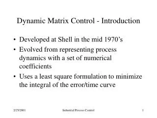
Introduction • Model predictive control (MPC) • Dynamic matrix control (DMC; Cutler and baker , 1979) • An extension of DMC to handle constraints explicitly as linear inequalities was introduced by Garcia and Morshedi (1986) and denoted as quadratic dynamic matrix control (QDMC). • Garcia (1984) proposed an extension of QDMC to nonlinear processes.
Linear and nonlinear QDMC • Linear QDMC utilizes a step or impulse response model of the process, and NLQDMC utilizes the model of the process represented by nonlinear ordinary differential equations. • These approximations are necessary in order for the on-line optimization to be a single QP at each sampling point.
Algorithm formulation with state estimation • For the general caseof MIMO systems, consider process and measurement models of the form • where xis the state vector, yis the output vector, uis the vector of manipulated variables, and w~ (0, Q)and u ~(0, R) are white noise. Qand Rare covariance matrices associated with process and measurement noise
Algorithm formulation with state estimation(cont’d) • Know at Sampling Instant k: y(k)the plant mea-surement, the estimate of state vector at kbased on information at k-1, and u(k-1)the manipulated variable.
Effect of future manipulated variables • Step 1: Linearize the at and u(k-1)to obtain where
Effect of future manipulated variables(cont’d) • Step 2: Discretize above equations to obtain • where Fkand Gkare discrete state space matrices (e.g., Åström and Wittenmark, 1984), obtained from Ak, Bk, and the sampling time.
Effect of future manipulated variables(cont’d) • Step 3: Compute the step response coefficients Si,k(i = 1, 2,..., P)where P is the prediction horizon. Si,kcan be obtained from • Step response coefficients can also be obtained by numerical integration of the linearized model over P sampling intervals with u = 1.0and x (tk)= 0.0 where tk isthe time at any sampling point k.
Computation of filter gain • Step 4: Compute the steady-state Kalman gain using the recursive relation (Åström and Wittenmark, 1984): • where Pjkis the state covariance at iteration jfor the model obtained by linearization at sampling point k. P∞kis the steady-state value of state covariance for that model.
Effect of past manipulated variables • Step 5: The effect of past inputs on future output predictions, y*(k+1), y*(k+2), ..., y*(k+P)is computed follows. Here the superscript * indicates that input values in the future are kept constant and equal to u(k-1). • Set • Define • Assume • For i = 1, 2,..., P, successively integrate over one sampling time from , with and then add to obtain Addition of Kkdprovides correction to the state. We can then write
Output prediction • Step 6: The predicted output is computed as the sum of the effect of past and future manipulated variables and the future predicted disturbances. Future disturbances Past effect Future effect
Optimization • Optimization. • where P is the prediction horizon • Mis the number of future moves • It is assumed that u(k+M-1)= u(k+M)= ... = u(k+P-1). • G and Lare diagonal weight matrices.
Optimization(cont’d) • The above optimization problem with constraints can be written asa standard quadratic programming problem: Subject to where and D and b depend on the constraints on manipulated variables, change in manipulated variables, and outputs.
Estimation of state • Step 7: The Mfuture manipulated variables are computed, but only the first move is implemented (Garcia and Morshedi, 1986). • Estimation of State. • Step 8 : Integrate from and u(k)over one sampling time and add Kkdto obtain
Example • For the reaction A + B↔P the rate of decomposition of B is • The system is described by a dynamic model of the form:
Example(cont’d) • Isothermal CSTR
Example(cont’d) • u1is the inlet flow rate with condensed B, • u2 is the inlet flow rate with dilute B, • x1 is the liquid height in the tank, • x2is the concentration of B in the reactor. • The control problem is simulated with the values • k1= 1.0, k2= 1.0, • CB1 = 24.9, and CB2 = 0.1.
Multi-equilibrium points at steady state • Multi-equilibrium points of CB At u1=1.0, u2=1.0 Lower steady state α=[ 100, 0.6327 ] Middle steady state β=[ 100, 2.7870 ] Upper steady state γ=[ 100, 7.0747 ]
Simulation results • A setpoint change from an initial condition of xl0 = 40.00and x20= 0.1to the unstable steady-state point with values at x1 = 100.00and x2 = 2.787. • The lower bounds on u1and u2are kept at zero • The upper bounds varied from 5, 10 to ∞ • A sampling time Ts = 1.0min • Tuningparameter values P = 5 and M = 5 • For the tuning parameter L= diag[0.0,0.0], G = diag[1.0,1.0]
Simulation results(cont’d) • The plant is running at the unstable steady state. Consider a step disturbance of 0.5 unit in u1. • A sampling time Ts = 1.0 min • the tuning parameter values P = 5.0, M = 5.0, L = 0.0, u10= 1.0 and u20= 1.0 are used in the simulations. • The lower bounds on u1and u2are kept at zero, and there are no upper bounds.
Tuning parameters • System parameter • Sampling time • Tuning parameters • Prediction horizon • Longer horizons tend to produce more aggressive control action and more sensitive to disturbances. • Control horizon • Shortening the control horizon relative to the prediction horizon tend to produce less aggressive controllers, slower system response and less sensitive to disturbances • Penalty weights
Some problems of NLQDMC • Truncation error in NLQDMC • Different sampling times • If system has large different responses in each loop • Tuning problem in NLQDMC
Conclusion • The proposed algorithm stabilizes open-loop unstable plants and The incorporation of a Kalman filter also results in better disturbance rejection when compared to Garcia's algorithm. • The major advantage of the proposed algorithm compared to the nonlinear programming approaches is that only a single quadratic program is solved on-line at each sampling time. • The use of the software package CONSOLE can obtain solution to an off-line optimization to tune the NLQDMC parameters.