Sampling and estimation

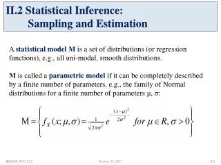
1. Statistics Applied to Bioinformatics Sampling and estimation Jacques.van.Helden@ulb.ac.be Laboratoire de Bioinformatique des Génomes et des Réseaux Université Libre de Bruxelles, Belgique

2. Overview: sampling and estimation • Definitions • Population and sample • Random sampling • Expectation • Sampling distributions • Sample mean • Sample median • Sample variance • Estimation • Population mean • Population median • Using sample median to estimate population mean • Population variance • Confidence limits • Population mean • Population median • Population varianc

3. Population and sample • Let us have a population of N elements, N being large. • We select a sample of n elements in the population. • We measure a certain characteristics on each element of the sample, and we obtain the sample values. Population (N elements) Sample (n elements)

4. Examples of samples and populations • Saccharomyces cerevisiae genome • The 3rd chromosome (sequenced in 1991) was a sample of the whole genome (sequenced in 1996) • Human genome • The first human genome ever sequenced was a sample of 1 element taken from a population of 6 billion elements. • 1000 human genomes: project announced in 2008. A sample of 1000 genomes in a population of 6 billion human genomes. • Microarray expression profiling of cancer tissues • Expression profiles taken from 30 patients suffering from a given cancer type. • Each tissue sample is a subset of cells of the cancerous tissue/organ. • Each patient is a sample of a population of all the persons suffering from the same cancer type in the world.

5. Example of the yeast genome • In 1991, first eukaryote chromosome completely sequenced: the chromosome III from the yeast Saccharomyces cerevisiae. • Sequence length: 316,616 bp • 173 ORFs • We can consider this as a sample taken from a larger population (the set of all ORFS on the 16 yeast chromosomes), still unknown at that time. • In 1996: the first eukaryote genome completely sequenced: Saccharomyces cerevisiae • 6,310 polypeptides (this can be considered as the population) • 16 chromosomes • Total size: 12,156,590 bp

6. Estimating a parameter of the population from a sample • On the basis of the sample, we want to estimate some parameters of the population. • E.g.: mean, standard deviation. Population (N elements) Sample (n elements)

7. Estimating a parameter of the population from a sample • Would we have chosen another sample, the sample mean and standard deviation would have been different. • The population mean and standard deviation are however constant. • Question: to which extent can we rely on the mean and standard deviation of the sample to estimate the mean and standard deviation of the population ? Population (N elements) Sample (n elements)

8. Expectation • Where • P(x) is the probability to observe the value x (discrete random variables) • f(x) is the density function (continuous random variables) • f(x)dxis an element of probability • y(x) can be any function of the random distribution x, The mean, the variance, the median, ... • E(Y) is called the expectationfor the random variable Y defined by the function y(x). Continuous variables Discrete variables

9. Sampling distribution of the mean • Take r samples, each of size n • For each sample (x1,x2,...,xn), calculate the mean • Each sample will have its own mean • How big is the dispersion of the mean values ? • What is the mean value of the mean ? • What is the distribution of the mean ?

10. Sampling distribution of the mean

11. Sampling distribution of the mean • In this simulation, the population is drawn randomly from a uniform distribution. • When the sample size (n) increases, the sample mean tends towards a normal distribution. This is an application of the central limit theorem. • On the histograms of the previous slide, the distribution of the sample means is always centred around 0.5, irrespective of the sample size. The mean of the sample is an unbiased estimate of the population mean: its expected value equals the mean of the population. • The variance and standard deviation of the sample mean decrease as the sample size (n) increase.

12. Sampling distribution - Sample variance • The sample variance is a biased estimator of the population variance. • For this reason, one has to introduce a corrective factor when one tries to estimate the population variance from the sample variance. • Remarks • This correction only matters for small samples. For large samples, n/(n-1) ~ 1. • This correction is already included in some packages (e.g. R): when you ask for the variance of a vector, it returns the estimate for population variance.

13. Sampling distribution - The standard error • The expectation for the sample mean is the population mean. The sample mean is thus an unbiased estimator of the population mean. (the hat means "estimate") • The variance of the sample mean distribution differsfrom the population variance. for a finite population for an infinite population • The standard deviation of the sample mean is called standard error. The standard error decreases when n increases. The larger is the sample, the more reliable is the estimation of the mean. for a finite population for an infinite population

14. Standard error - simulation • We generated 20,000 random samples with a normal distribution N(0,1), and calculated the distribution of their means, for various sample sizes (n) • The dots show the distribution of sample mean, for each sample size. • The lines show the theoretical distribution, i.e. N(0, 1/sqrt(n))

15. Sampling distribution – Sample median • The expectation for the sample median is the population median. The sample median is thus an unbiased estimator of the population median • In the case of symmetric populations, • The sample median is also an unbiased estimator of the population mean • The sample median is less efficient in the sense that its variance is higher than the variance of the sample mean. However it is more robust to the presence of outliers. When the sample is suspected to contain outliers, the sample median is thus preferable. This is typically the case with microarray data.

16. Statistics Applied to Bioinformatics Confidence interval around the mean Jacques.van.Helden@ulb.ac.be Laboratoire de Bioinformatique des Génomes et des Réseaux Université Libre de Bruxelles, Belgique

17. Back to 1991 • Let us suppose that we are back in 1991 • We have a sample of 173 sequences (all ORFs from the chromosome III). • We would like to infer from this sample some characteristics of the population (the complete genome) • Mean gene length • Variance of gene length • Questions: • How can we estimate the mean length of all yeast ORFs ? • Can we define a confidence interval around our estimation ? • How can we estimate the variance of all yeast ORF lengths ? • Can we define a confidence interval around this estimation ? • After having performed these estimation, we will jump from 1991 to 1996 and evaluate our estimations.

18. Confidence interval around the mean with a pre-defined variance • The confidence interval is defined as a range around the mean estimate, having a probability 1- to include the mean • BEWARE • The mean of a population (m) is NOT a stochastic event. Its value is defined by the population. • It is thus INCORRECT to say that “m has a X% probability to fall within the confidence interval” • The probability is a property of the interval : we can say that the interval [x1,x2] has a probability of 95% to include the mean. • When the variance is known a priori, the confidence interval around the mean can be estimated using the normal distribution, with the standard error as parameters of dispersion. • Exercise • search in the normal table the value of u corresponding to risk of error of 5% • Warning • usually, the variance is a priori not known, see next slide

19. Confidence interval around the mean when the population variance has to be estimated from the sample itself • In most practical cases, the variance is priori not known. • The population variance has thus to be estimated from the sample variance. • This introduces an error, which modifies the theoretical distribution. • Instead of a normal, use a Student distribution with k=n-1 degrees of freedom. • In practice, the Student distribution tends towards a normal when n.

20. 1991: parameters for the 173 ORFS on the basis of the 3rd chromosome

21. 1991: estimating parameters about genome on the basis of the 3rd chromosome

22. 1991: confidence interval around ORF length

23. 1996: we can check the prediction