Truncation Errors and the Taylor Series Chapter 4
190 likes | 546 Vues
Truncation Errors and the Taylor Series Chapter 4. How does a CPU compute the following functions for a specific x value? cos (x) sin(x) e x log(x) etc.

Truncation Errors and the Taylor Series Chapter 4
E N D
Presentation Transcript
How does a CPU compute the following functions for a specific x value? cos(x) sin(x) ex log(x)etc. • Non-elementary functions such as trigonometric, exponential, and others are expressed in an approximate fashion using Taylor series when their values, derivatives, and integrals are computed. • Taylor series provides a means to predict the value of a function at one point in terms of the function value and its derivatives at another point.
Taylor Series (nth order approximation): The Reminder term, Rn, accounts for all terms from (n+1) to infinity. Define the step size as h=(xi+1- xi), the series becomes:
Any smooth function can be approximated as a polynomial. Take x = xi+1 Then f(x) ≈ f(xi) zero orderapproximation first orderapproximation Second orderapproximation: nth orderapproximation: • Each additional term will contribute some improvement to the approximation. Only if an infinite number of terms are added will the series yield an exact result. • In most cases, only a few terms will result in an approximation that is close enough to the true value for practical purposes
ExampleApproximate the function f(x) = 1.2 - 0.25x- 0.5x2 - 0.15x3 - 0.1x4 from xi = 0 with h = 1 and predictf(x) at xi+1 = 1.
Example: computing f(x) = ex using Taylor Series expansion Choose x = xi+1and xi = 0 Then f(xi+1) = f(x) and(xi+1 – xi)= x Since First Derivative of ex is also ex : (2.) (ex )” = ex (3.)(ex)”’ = ex, … (nth.)(ex)(n) = ex As a result we get: Looks familiar? Maclaurin series for ex
Yet another example: computing f(x) = cos(x) using Taylor Series expansion Choose x=xi+1 and xi=0 Then f(xi+1) = f(x) and (xi+1 – xi) = x Derivatives of cos(x): (1.) (cos(x))’ = -sin(x)(2.) (cos(x) )” = -cos(x), (3.) (cos(x) )”’ = sin(x) (4.) (cos(x) )”” = cos(x), …… As a result we get:
Notes on Taylor expansion: • Each additional term will contribute some improvement to the approximation. Only if an infinite number of terms are added will the series yield an exact result. • In most cases, several terms will result in an approximation that is close enough to the true value for practical purposes • Reminder value R represents the truncation error • The order of truncation error is hn+1 R=O(hn+1), If R=O(h), halving the step size will halve the error. If R=O(h2), halving the step size will quarter the error.
Error Propagation • Let xfl refer to the floating point representation of the real number x. • Since computer has fixed word length, there is a difference between x and xfl (round-off error) and we would like to estimate the error in the calculation of f(x) : • Both x and f(x) are unknown. • If xfl is close to x, then we can use first order Taylor expansion and compute: Result: If f’(xfl) and Dx are known, then we can estimate the error using this formula Solve from Example 4.5 p.95