Work Done : ~6/03/03

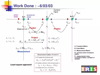
1. Work Done : ~6/03/03 Control Input priori state posteriori state k+1 k-1 k Predict Predict State at t=k-1 Project A: Transition Matrix B: Scale Matrix H : Measurement Matrix Q - process noise covariance matrix, R - measurement noise covariance matrix, constant or variable Measurement Least-square approach

2. How to calculate each parameter? Example : Suppose x has 2 dimensions at each time- position(a,b) Q= measurement noise [0.1 0 0 0.1] Usually constant -> Ideally variable R= Process noise [0.1 0] Usually constant -> Ideally variable H= measurement matrix [1 1 ] A= [1 0 0 1] 2*2 matrix – Usually constant -> Ideally variable B= Scale matrix If no input -> 0 X1 = [1 ;1] X3 = [? ;?] X2 = [2 ; 5] Initial State k+1 k-1 k [1; 1] [1.2530 ; 1.2530 ] Predict Predict K =[0.03 0.02 0.03 0.02 ] [0.1 0 0 0.1] Z=[7.1 ; 7.0] [1.2530 1.2530]

3. Live Demo from OpenCV Output of each parameter White cross : current state Red cross : measurement Green cross : Predicted state

4. Work Done : ~5/21/03 zk=H•xk+vk measurement A priori state least square approach was used A posteriori state Example : Suppose x has 4 dimensions at each time- position(a,b) and velocity (c,d) A= [1 0 1 0 0 1 0 1 0 0 1 0 0 0 0 1] 4*4 matrix – Usually constant -> Ideally variable Q= measurement noise [0.1 0 0 0 0 0.1 0 0 0 0 0.1 0 0 0 0 0.1] Usually constant -> Ideally variable B= Scale matrix If no input -> 0 R= Process noise [0.1 0 0 0 0 0.1 0 0 0 0 0.1 0 0 0 0 0.1] Usually constant -> Ideally variable H= measurement matrix [1 0 0 0 0 1 0 0] Usually constant -> Ideally variable( n*4, here n=2)

5. Discrete Kalman Filter Examples

6. More kalman filters • Discrete Kalman Filter – Linear stochastic difference equation Propagation of a Gaussian random variable (GRV) • Square-root Kalman Filter • Continuous-Kalman Filter • Extended Kalman Filter – Nonlinear stochastic difference equation The state distribution is approximated by a GRV, which is then propagated analytically through the first-order linearization of the nonlinear system • Unscented Kalman Filter (UKF) The UKF addresses the approximation issues of the EKF. The state distribution is again approximated by a GRV, but is now represented using a minimal set of carefully chosen sample points • Kalman Adaptive Filter

7. Directions for Future work? • Implementation of Kalman filter with video tracking • Needs more investigation with several Kalman Filters and Condensation Algorithm?

8. Work Done : ~5/7/03 Kalman Filter Images from Welch 1995

9. Kalman Filter Algorithm http://www.spd.eee.strath.ac.uk/users/was/project/Theory/Kalman.htm

10. Kalman Filter Algorithm http://www.spd.eee.strath.ac.uk/users/was/project/Theory/Kalman.htm

11. Kalman Filter in the OpenCV xk=A•xk-1+B•uk+wk zk=H•xk+vk, where: xk (xk-1) - state of the system at the moment k (k-1) zk - measurement of the system state at the moment k uk - external control applied at the moment k wk and vk are normally-distributed process and measurement noise, respectively: p(w) ~ N(0,Q) p(v) ~ N(0,R), that is, Q - process noise covariance matrix, constant or variable, R - measurement noise covariance matrix, constant or variable

12. Kalman Filter in the OpenCV CvKalman{ int MP; /* number of measurement vector dimensions */ int DP; /* number of state vector dimensions */ int CP; /* number of control vector dimensions */  CvMat* state_pre; /* predicted state (x'(k)): x' (k)=A*x(k-1)+B*u(k) */ CvMat* state_post; /* corrected state (x(k)): x(k)=x'(k)+K(k)*(z(k)-H*x'(k)) */ CvMat* transition_matrix; /* state transition matrix (A) */ CvMat* control_matrix; /* control matrix (B) (it is not used if there is no control)*/ CvMat* measurement_matrix; /* measurement matrix (H) */ CvMat* process_noise_cov; /* process noise covariance matrix (Q) */ CvMat* measurement_noise_cov; /* measurement noise covariance matrix (R) */ CvMat* error_cov_pre; /* priori error estimate covariance matrix (P'(k)): P'(k)=A*P(k-1)*AT+ Q)*/ CvMat* gain; /* Kalman gain matrix (K(k)): K(k)=P'(k)*HT*inv(H*P'(k)* HT +R)*/ CvMat* error_cov_post; /* posteriori error estimate covariance matrix (P(k)): P(k)=(I-K(k)*H)*P'(k) */ CvMat* temp1; /* temporary matrices */ CvMat* temp2; CvMat* temp3; CvMat* temp4; CvMat* temp5; } CvKalman;

13. Kalman Filter related functions • cvCreateKalman : Allocates Kalman filter structure • cvReleaseKalman :Deallocates Kalman filter structure • cvKalmanPredict : Estimates subsequent model state x'k=A•xk+B•uk P'k=A•Pk-1*AT + Q, where x'k is predicted state (kalman->state_pre), xk-1 is corrected state on the previous step (kalman->state_post) (should be initialized somehow in the beginning, zero vector by default), uk is external control (control parameter), P'k is priori error covariance matrix (kalman->error_cov_pre) Pk-1 is posteriori error covariance matrix on the previous step (kalman->error_cov_post) (should be initialized somehow in the beginning, identity matrix by default) • cvKalmanCorrect : Adjusts model state Kk=P'k•HT•(H•P'k•HT+R)-1 xk=x'k+Kk•(zk-H•x'k) Pk=(I-Kk•H)•P'k where zk - given measurement (mesurement parameter) Kk - Kalman "gain" matrix.

14. Live Demo 1 from OpenCV White cross : current state Red cross : measurement Green cross : Predicted state White cross and green cross are merge together -> Best prediction

15. Live Demo 2 White cross : current state Red cross : measurement Green cross : Predicted state

16. Work Done : ~4/23/03 xk=A•xk-1+B•uk+wk zk=H•xk+vk, where: xk (xk-1) - state of the system at the moment k (k-1) zk - measurement of the system state at the moment k uk - external control applied at the moment k wk and vk are normally-distributed process and measurement noise, respectively: p(w) ~ N(0,Q) p(v) ~ N(0,R), that is, Q - process noise covariance matrix, constant or variable, R - measurement noise covariance matrix, constant or variable

17. Discrete Kalman Filter - PDF A priori state A posteriori state estimate A Priori estimate error covariance A posteriori estimate error covariance Measurement covariance error Images from Welch 1995

18. Discrete Kalman Filter Examples Images from http://www.ai.mit.edu/~murphyk/Software/Kalman/kalman.html

19. Extended Kalman Filter Images from Welch 1995

20. Next week • Survey on Kalman filter • Applications • Detail analysis of Kalman filter algorithm • (http://www.cs.unc.edu/~welch/kalman/index.html#Anchor-49575)

21. Work Done : ~4/09/03 Condensation : Conditional Density Propagation • Uses ``factored sampling'', previously applied to the interpretation of static images, in which the probability distribution of possible interpretations is represented by a randomly generated set. • Uses learned dynamical models, together with visual observations, to propagate the random set over time. • Applied in many applications such as multiple objects tracking • Many advantages than Kalman Filtering • Kalman filtering have been used for tracking, but such methods can only model unimodal probability distributions and thus cannot form alternative hypotheses about the location of the object being tracked

22. Condensation Algorithm - PDF • Overview of Condensation (from Isard and Blake, IJCV 1998): Define xt to be the state of the object being modeled (and tracked) at time t and zt to be the set of image features observed at time t. • From the "old" sample-set { st-1[n], wt-1[n], ct-1[n], n=1..N } at time-step t-1, construct a "new" sample-set { st[n], wt[n], ct[n], n=1..N } for time t. • Construct the nth of N new samples as follows: • Select a sample s't[n] as follows: • generate a random number r in [0,1], uniformly distributed. • find, by binary subdivision, the smallest j for which ct-l[j] >= r • set s't[n] = st-l[j] • Predict by sampling from p(xt | xt-1 = s't[n]) to choose each st[n]. • Measure and weight the new position in terms of the measured features zt: wt[n] = p(zt | xt = st[n]) then normalize so that Sum(wt[n] over n) = 1 and store together with cumulative probability as (st[n], wt[n], ct[n]) where ct[0] = 0,ct[n] = ct[n-1] + wt[n] for (n = 1..N). • Once the N samples have been constructed, estimate the mean tracked position as xmean(t) = Sum(wt[n] * st[n] over n)

23. Condensation Examples Movies From http://www.dai.ed.ac.uk/CVonline/LOCAL_COPIES/ISARD1/condensation.html

24. Next Week • Next week : • Study Condensation algorithm in detail ( Theory, Mathematical, Extension of basic algorithms to application) • Summary of Literature

25. Work Done : ~4/03/03 Condensation : Conditional Density Propagation • Uses ``factored sampling'', previously applied to the interpretation of static images, in which the probability distribution of possible interpretations is represented by a randomly generated set. • Uses learned dynamical models, together with visual observations, to propagate the random set over time. • Applied in many applications such as multiple objects tracking • Many advantages than Kalman Filtering

26. Literature Survey • Zhao 2002, Face Recognition from Video: A Condensation Approach • Isard et al 1998, CONDENSATION – Conditional density propagation for visual tracking • Black et al 1998, Recognizing Temporal Trajectories using the Condensation Algorithm • Meier et al 1998, Using the Condensation Algorithm to Implement Tracking for Mobile Robots • Isard 1996, Contour tracking by stochastic propagation of conditional density ( Origin) • Next week : • Study Condensation algorithm in detail ( Theory, Mathematical, Extension of basic algorithms to application, Comparison with Kalman Filtering) • Summary of Literature

27. Work Done : ~3/12/03 Head-Region Extraction Using Direct-Least Square Ellipse Fitting -Works well. Can be improved by Background Subtraction - Processing individual frames ( Not using optical flow) Decision needed for future work ( Which direction) - A lot of methods • Tracking ( Head, and eyes) – Consistency of individuals • Face detection ( Eye distance) • Facial feature detection ( Eyes, nose, and mouth) • Face recognition ( Features extraction) Literature review • Elliptical Head Tracking using Intensity gradients and Color Histograms (Birchfield 98) – Color information is added • Face Detection and Precise Eyes Location ( Huang 2000)

28. Literature Review: Face Detection and Precise Eyes Location • Pre-attentive feature detection : 2nd derivative Gaussian Filter -The response is a peak or valley in the center of features (Multi scale with multi orientation filter) • Facial image analysis : • Structure Model • Texture Model : Measures the gray or color similarities of a candidate with face model -> Chin areas were used • Feature Model : Eigen-eye with image feature analysis

29. Literature Review: Cont’d • Precise Eye Location : Reduce greatly the number of the scales under consideration during the recognition. • Preprocessing (Edge Detection) • Light cancellation • Circular Detection • ( Hough & Circular Correlation) • Region Homogeneity ( Eyeball ) – Homogeneous, Darker than white region surrounding it.

30. Literature Review: Cont’d • Selecting Best Center ( The distance between the eyes are 100 pixels) • Selecting Best Candidates Next Week • Assist Video tracking demo if necessary • Which Directions ? • After detecting faces -> Truefaces (From Leading Edge) will be used for Face Recongtion

31. Work Done : ~2/26/03 Head-Region Extraction Using Direct-Least Square Ellipse Fitting • Direct-Least Squares Fitting Ellipses • Canny Edge Detector from Video Sequences • Select Best Candidates • Experimental Results Direct-Least Squares Fitting Ellipses -> Original Paper • Least-Squares conic fitting is used for ellipse fitting -> but it can lead to other conics ( Iterative ) • Direct Least-Squares Non-iterative ellipse fitting • Yields best LSQ ellipse fit • Robust to noise

32. Background : Conic Fitting Implicit equation of a conic Least square algebraic fitting Eigenvalue Fitting (if constraint is quadratic) C: Contraint matrix

33. Background : Conic Fitting Previous Methods Direct Least-Squares Methods

34. Results using Direct LSQ

35. Results using Direct LSQ Edge detector -> Canny (Frame difference is not good) Ignore small ellipse

36. Results using Direct LSQ from Video If there are elliptical shapes, it detects well. Background should be removed for better performance. Usually chin regions have weak edges, it may not be detected well -> If chin regions are detected, we can acquire more accurate ellipses.

37. Next Week • Background Extraction • Experiment elliptical fitting of head using several video sequences from airport and Ferris hall • Study on other methods • Elliptical Head Tracker(Birchfield 97) • Elliptical Head Tracking using Intensity gradients and Color Histograms (Birchfield 98)

38. Work Done : ~2/19/03 • Implementation of face detection using OpenCV • Study on Curve-fitting methods • Direct Least-Square for Ellipse Fitting for extracting for head-region - Not good at this time (Using Frame Difference and Edges)

39. Next Week • Survey on Detecting Interesting Points. • Develop Direct Least-Square for Ellipse Fitting for extracting for head-region