Introduction to frequency analysis, IDF and Design storms
500 likes | 679 Vues
Introduction to frequency analysis, IDF and Design storms. Ir. Gabriel Parodi WRS- ITC 2010. Events and extreme events. “Man can believe the impossible. But man can never believe the improbable.” - Oscar Wilde.

Introduction to frequency analysis, IDF and Design storms
E N D
Presentation Transcript
Introduction to frequency analysis, IDF and Design storms Ir. Gabriel Parodi WRS- ITC 2010
Events and extreme events “Man can believe the impossible. But man can never believe the improbable.” - Oscar Wilde “It seems that the rivers know the [extreme value] theory. It only remains to convince the engineers of the validity of this analysis.” –E. J. Gumbel
Hazard = Probability of event with a certain magnitude Concept of Risk • RISK = HAZARD * VULNERABILITY * AMOUNT Intensity Frequency Duration
Magnitude-frequency relation • Disasters generally follow the magnitude – frequency relation, which means that events with a smaller magnitude happen more often than events with large magnitudes.
Magnitude – frequency relations • Irregular • Random • Log-normal • Seasonal • Diurnal • Etc…
1 ABSOLUTE CERTAINTY That you will die some day 0.9 0.8 0.7 That you ( a man) will be taller than 1.70 m. 0.6 Probability scale 0.5 That a coin will come down heads 0.4 0.3 0.2 That you will win the lottery 0.1 0 That you can swim across the Atlantic ABSOLUTE IMPOSSIBILITY Probability Probability may be described as the relative frequency with which an event occurs or will occur in the long run. It is measured normally on a scale ranging from 0 (meaning impossible) to 1 (meaning certain)
Some terms… • Hazard: Probability that a particular danger (threat) occurs within a given period of time. • Likelihood: Conditional probability of an outcome given a set of data, assumptions and information. Also used as a qualitative description of probability and frequency. • Probability:A measure of the degree of certainty. This measure has a value between zero (impossibility) and 1.0 (certainty). It is an estimate of the likelihood of the magnitude of the uncertain quantity, or the likelihood of the occurrence of the uncertain future event. • Annual exceedance probability (AEP):The estimated probability that an event of specified magnitude will be exceeded in any year.
12 10 8 Frequency 6 4 2 0 800 450 500 550 600 750 850 900 950 650 700 Rainfall classes (mm) Frequency Analysis
X Frequency Analysis P(R < 642) = 0.5 Mean: 642 mm Standard deviation: 110 mm P(R > 642) = 0.5 P(532 < R < 752) = 0.683 P(422 < R < 862) = 0.954 P(312 < R < 972) = 0.997 0.683 0.954 0.997 -2 +2 -3 -1 +1 +3
Frequency Analysis Distribution Real data 50 occurrences (n=50) Expected Actual P(R < 642) = 0.5 25 29 25 21 P(R > 642) = 0.5 P(532 < R < 752) = 0.683 34 36 P(422 < R < 862) = 0.954 48 48 50 P(312 < R < 972) = 0.997 50
100 80 Cumulative % 60 40 20 0 800 450 500 550 600 750 850 900 950 650 700 Rainfall classes (mm) Frequency Analysis
Frequency Analysis Cumulative probability curve for a normal distribution 1 0.8 0.6 Cumulative probability 0.4 0.2 0 Avg+1STD Avg-2STD Avg-1STD Avg+2STD Avg
Frequency Analysis Straightened cumulative probability curve for a normal distribution Normal probability paper 0.977 0.84 0.5 Cumulative probability 0.16 0.022 Log (Avg+1STD) Log (Avg-2STD) Log (Avg-1STD) Log (Avg) Log (Avg+2STD)
12 10 8 Frequency 6 4 2 0 800 450 500 550 600 750 850 900 950 650 700 Rainfall classes (mm) Right skewed: very important Large amount of events are right skewed; • Magnitude of events are absolutely limited at the lower end and not at the upper end. The infrequent events of high magnitude cause the characteristic right-skew. • The closer the mean to the absolute lower limit, the more skewed the distribution become. • The longer the period of record, the greater the probability of infrequent events of high magnitude, the greater the skewness. • The shorter the time interval of recording, the greater the probability of recording infrequent events of high magnitude, the greater the skewness. • Other physical principles tend to produce skewed frequency distributions: e.g. drainage basin size versus size of high intensity thunderstorms.
3 1 1 5 Between 1935 and 1978: 9 events 6 8 Intervals, ranging from 1 to 16 years 16 5 4 Frequency analysis (0-D) Maximum daily preciptation (mm) What is the return period of a rain event over a 100 mm/day ? The sum of the intervals = 4 + 1 + 1 + 16 +3 + 6 + 5 + 5 = 41 Average = 41/8 = 5.1 years Annual exceedence probability of a rain event over 100 mm/day = 100 / 5.1 = 19.5 %
Relation between Probability and Return period • What is the probability ‘p’ that in a certain period of time (i.e. 1 year), the intensity of one event ‘X’ (rainfall) of duration ‘d’ (hours or days) is bigger than ‘xt’ (100 mm)? • P(X>100) when X is rainfall of i.e. 24 hs duration expressed in mm. • Notice that this is applicable for any other durations. • We assume that the events are independents • So we start observing events. You wait for (1 year) and you note down the rainfalls in this year. For each year observation, there are two possible outcomes • “success" X xt (probability p) • "failure" X < xt (probability 1-p) • Since the observations are independent, the probability of a recurrence interval of duration T (1 year) is the product of the probabilities of (T-1) failures followed by one success: • First year: failure -> (1-p) • Second year: failure -> (1-p) • Third year: failure -> (1-p) • Forth year: Success!! -> p • So the probability of success in general is (1-p)*(1-p)*(1-p)*p= (1-p)(t-1) * p • Assuming that the series of data is infinite, the E(T) can be expressed as: • This is equal to: • So, the probability of occurrence of an event in any observation is the inverse of its return period.
Extreme value distributions • Of a series you take the maximum or minimum observations of independent periods. (largest flow per year). • The general form of the probability distribution of extremes that summarizes all cases is where z=(x-μ)/σ, and k, σ, μ are the shape, scale, and location parameters respectively.: • The cumulative probability function, the integral of the previous function is: • Based on the value of ‘k’ there are three extreme value equation types (I, II, III).
Extreme value type I: Gumbel distribution • Medium tailed • In this case k → 0. 2 parameters!! • The function is not bounded and X is real number. • The shape of the Gumbel model does not depend on the distribution parameters. • The parameters are calculated from the data, where sx is the standard deviation of the sample.
Extreme value type II: Frechet distribution • Long tailed • In this case k < 0. Three parameters. • α is the shape parameter (α>0), and β is the scale parameter (β>0). • This distribution is bounded on the lower side (x>0) and has a heavy upper tail. The animation below shows the Fréchet PDF graph for β=1 and various values of α:
Extreme value type III: Weinbull distribution • Short tailed • In this case k > 0. Three parameters. • The Weibull distribution is defined for x>0, and both distribution parameters (α - shape, β - scale) are positive. • The function is bounded, it is valid for x < u. the functions is equal to 1 for x>= u • Gumbel and Fréchet models described above relate to maxima (largest extreme value), while the Weibull model relates to minima (smallest extreme value)
Gumbel method Solution: • Use Extreme Value transform • Rank the values from the smallest to the largest value. • Calculate the cumulative probabilities: P=R/(N+1) • Plot the values against the cumulative probability on probability paper and draw a straight line (best fit) through the points • From the line, estimate the standard deviation and mean • Estimate all other required probabilities versus values
Sequence in excel Rank/(N+1) 1/(1-left prob)
Q = 79000 -> Plot -> Prob -> TR Plot -> Prob -> TR. Q from the interpolation Graph and operation plot = 7E-05 Q - 3.1277 Q = 79000 -> Plot -> Prob -> TR =1/(1-Prob) EXP(-EXP(-plot))
Frequency Analysis Suppose a certain flood has a probability of occurrence of 10% PR (F) = 0.10 In the long run, the flood would occur on the average once in 10 years. Thus the average return period T (in years) is defined as: T = 1/PR(F) The probability that F will occur in a any year: PR(F) = 1/T The probability that F will NOT occur in any year: PL(F) = 1 - PR(F) = 1 - 1/T The probability that F will NOT occur in any of n successive year: PLn(F) = (1 - 1/T)n The probability R (called RISK) that F will occur at least once in n successive year: R = 1- (1 - 1/T)n
Return period / exceedance probability. For the average annual risk! Q100 has a greater probability of occurring during the next 100 yrs (63%) than during the next 5 years ( 5%)
Some software • Extremes toolkit • http://www.isse.ucar.edu/extremevalues/extreme.html • The Extremes Toolkit consists of functions written in "R" to perform extreme value analysis • XTREMES software • http://www.xtremes.de/xtremes/index.htm • Software for extreme value statistics
Books and notes on statistics of extremes • An Introduction to Statistical Modeling of Extreme Valuesby Stuart Coles (Springer, 2001) • Statistical Modeling of Extreme Values from Insurance, Finance, Hydrology, and Other Fieldsby R.-D. Reiss and M. Thomas (Birkhauser, Second Edition, 2001) • Lecture notes on environmental statistics by Richard Smith (see Chapter 8 on extremes)
Point rainfall to areal rainfall • If a certain rainfall fall at a point, how much is fallen in the catchment? • For a catchment, the extrapolation is expected to get a reduction. • Realistic rainfall runoff modeling requires better estimation of the areal rainfall.
Reduction methods: depth-area-duration • For the general case, Depth-area relationships for various durations, are derived by a depth-area-duration analysis • Isohyetal maps are prepared for every duration from the tabulation of maximum n-hour rainfalls recorded in a densely gaged area. • The area contained within each isohyets on these maps is determined and a graph of average precipitation depth vs. area is plotted for each duration.
Reduction methods: depth-area-duration (2) • Factor of the US Weather bureau • Duration tr in hours and the area, A is in square miles. For example, if the average value of a 10-yr 6-hour rainfall at a certain place is 3.45 in., the average 6-hour depth over a drainage area of 200 mi • will be 85% of the point value, or 2.9 in.
Intensity Duration Frequency - IDF Ir. Gabriel Parodi WRS- ITC 2009
Working with duration, intensities and probabilities • Table shows the sequence of a rainfall event recorded every 5 minutes. In the last three columns the total of rainfall is grouped in intervals of 30, 60 and 120 minutes. • At the bottom the maximum depth in inches and maximum intensity in [inches/hour] is obtained. • For each duration, frequency analysis is performed on the data, as described in the section Gumbel Extreme value distribution. • This calculation is the basis for that defines the IDF curves graphs.
The approach to design storms: Intensity-duration-frequency (IDF) curves • One of the first steps in many hydrologic design projects is the determination of the rainfall event or events to be used. • The most common approach is to use a design storm or event that involves a relationship between rainfall intensity (or depth), duration, and the frequency or return period appropriate for the facility and site location. • In many cases, the hydrologist has standard intensity-duration-frequency (IDF) curves available for the site and does not have to perform this analysis. However, it is worthwhile to understand the procedure used to develop the relationships. • The intensity ‘I’ is the time rate of precipitation, that is, depth per unit time (mm/h or in/h). It can be either the instantaneous intensity or the average intensity over the duration of the rainfall. The average intensity is commonly used and can be expressed as: • where ‘P’ is the rainfall depth (mm or in) and Td is the duration, usually in hours. The frequency is usually expressed in terms of return period, T,
Example • Determine the design precipitation intensity and depth for a 20- minute duration storm with a 5-year return period. • Solution. From the IDF curves, the design intensity for a 5-year, 20-minute storm is i = 3.50 in/h. The corresponding precipitation depth is given by P= i*Td with Td = 20 min =0.333 h. • P= i*Td= 3.50* 0.333= 1.17 in.
Storm design • How we can design a storm for a structural design (Rain (time)) in a place? • Several methods depending on the data availability. As always, the more you know the more accurate the design.
From IDF: alternating block method • Design a 2 hours storm for a 10 minutes interval and for a return period of 5 years. • Table shows the sequence of calculation. Columns 1 and 2 are derived from the IDF, the other columns are calculations in sequence. • Column 7 is build centralizing in time the maximum depth and then assigning to each side the following ranked depths.
Design storms from observed temporal patterns • The major portion of a rainfall in one storm of a certain total duration falls in a short period of time. • So if “d” is the total duration of the storm, storms can be classified as based on the one-fourth of total storm time during which the greatest portion of rainfall occurred. • So storms can be in the first, second, third and fourth quartile. • The diagrams show the percentage of the total rainfall in the storm, associated to a certain percentage of the total duration of the storm, falling in the first quartile. • It has been observed that that for smaller areas (less than 10 square miles), the occurrence of precipitation was biased toward the beginning of the event. • For the first diagram, there is a 10% probability, that 52% of the total rainfall happens in the first 10% of the duration of he storm.
Design storms from observed temporal patterns (2) • The information here is for the first quartile. • For example, there is a 90 percent probability that approximately 60 percent of rainfall for a first quartile event occurs by 58 percent of the total storm duration. • Therefore, the 50 percent curve represents the media distribution of all observed first quartile events.
The NRCS Urban Hydrology for Small Watersheds (WINTR-55) prompts the user to enter the rainfall distribution type (I, Ia, II, or III), and then computes the direct surface runoff volume in inches and the peak runoff rate using the applicable 24-hour rainfall distribution. Different types of curves are built for different areas. Similar examples in models
Triangular method • A triangle is a simple shape for a design hyetograph because once the design precipitation depth P and a duration Td are known, the base length and height of the triangle are determined. • The base length is Td and the height h, so the total depth of precipitation in the hyetograph is given by P = 0.5.Td.h, so h=2.P/Td • A storm advancement coefficient r is defined as the ratio of the time before the peak ‘ta’ to the total duration td. R= ta/td • A value for r of 0.5 corresponds to the peak intensity occurring in the middle of the storm, while a value less than 0.5 will have the peak earlier and a value greater than 0.5 will have the peak later than the midpoint. A suitable value of r is determined by computing the ratio of the peak intensity time to the storm duration for a series of storms of various durations.