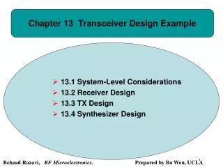
Chapter 13 Transceiver Design Example
Chapter 13 Transceiver Design Example. 13.1 System-Level Considerations 13.2 Receiver Design 13.3 TX Design 13.4 Synthesizer Design. Behzad Razavi, RF Microelectronics. Prepared by Bo Wen, UCLA. Chapter Outline. RX NF, IP 3 , AGC, and I/Q Mismatch TX Output Power and P 1dB

Chapter 13 Transceiver Design Example
E N D
Presentation Transcript
Chapter 13 Transceiver Design Example • 13.1 System-Level Considerations • 13.2 Receiver Design • 13.3 TX Design • 13.4 Synthesizer Design Behzad Razavi, RF Microelectronics. Prepared by Bo Wen, UCLA
Chapter Outline • RX NF, IP3, AGC, and I/Q Mismatch • TX Output Power and P1dB • Synthesizer Phase Noise and Spurs • Frequency Planning • Broadband LNA • Passive Mixer • AGC Synthesizer Design TX Design System-Level Specifications RX Design • VCO • Dividers • Charge Pump • PA • Upconverter
Receiver: Noise Figure 11a/g specifies a packet error rate of 10%. Since TX baseband pulse shaping reduces the channel bandwidth to 16.6 MHz, we return to and obtain for a sensitivity of -65 dBm (at 52 Mb/s). In practice, signal detection in the digital baseband processor suffers from nonidealities, incurring a “loss” of a few decibels. Moreover, the front-end antenna switch exhibits a loss of around 1 dB. • Manufacturers typically target an RX noise figure of about 10 dB.
Receiver: Nonlinearity We represent the desired, adjacent, and alternate channels by A0 cos ω0t, A1 cos ω1t, and A2 cos ω2t, respectively. For a third-order nonlinearity of the form y(t) = α1x(t) + α2x2(t) + α3x3(t), the desired output is given by α1A0cos ω0t and the IM3 component at ω0 by 3α3A12A2/4 We choose the IM3 corruption to be around -15 dB to allow for other nonidealities: • The IP3 corresponding to the 1-dB compression point is satisfied if compression by the desired signal is avoided. The IP3 arising from adjacent channel specifications must be satisfied while the desired signal is only 3 dB above the reference sensitivity.
Receiver: AGC Range • The receiver must automatically control its gain if the received signal level varies considerably. • The challenge is to realize this gain range while maintaining a noise figure of about 10 dB and an IIP3 of about -40 dBm. Determine the AGC range of an 11a/g receiver so as to accommodate the rate-dependent sensitivities. Solution: At first glance, we may say that the input signal level varies from -82 dBm to -65 dBm, requiring a gain of 86 dB to 69 dB so as to reach 1 Vpp at the ADC input. However, a 64QAM signal exhibits a peak-to-average ratio of about 9 dB; also, baseband pulse shaping to meet the TX mask also creates 1 to 2 dB of additional envelope variation. Thus, an average input level of -65 dBm in fact may occasionally approach a peak of -65 dBm+11 dB = -54 dBm. It is desirable that the ADC digitize this peak without clipping. That is, for a -65-dBm 64QAM input, the RX gain must be around 58 dB. The -82-dBm BPSK signal, on the other hand, displays only 1 to 2 dB of the envelope variation, demanding an RX gain of about 84 dB.
ACG Range: Required RX Gain Switching and NF and IIP3 Variations • The receiver gain range is also determined by the maximum allowable desired input level (-30dBm). The baseband ADC preferably avoids clipping the peaks of the waveforms. • The actual number of steps chosen here depends on the design of the RX building blocks and may need to be quite larger than that depicted
Example of AGC Range: Choice of Gain The choice of the gain in the above example guarantees that the signal level reaches the ADC full scale for 64QAM as well as BPSK modulation. Is that necessary? Solution: No, it is not. The ADC resolution is selected according to the SNR required for 64QAM modulation (and some other factors). For example, a 10-bit ADC exhibits an SNR of about 62 dB, but a BPSK signal can tolerate a much lower SNR and hence need not reach the ADC full scale. In other words, if the BPSK input is amplified by, say, 60 dB rather than 84 dB, then it is digitized with 6 bits of resolution and hence with ample SNR (≈ 38 dB) . In other words, the above AGC calculations are quite conservative.
Receiver: I/Q Mismatch • The I/Q mismatch study proceeds as follows. • (1) To determine the tolerable mismatch, we must apply in system simulations a 64QAM OFDM signal to a direct-conversion receiver and measure the BER or the EVM. Such simulations are repeated for various combinations of amplitude and phase mismatches, yielding the acceptable performance envelope. • (2) Using circuit simulations and random device mismatch data, we must compute the expected I/Q mismatches in the quadrature LO path and the downconversion mixers. • (3) Based on the results of the first two steps, we must decide whether the “raw” matching is adequate or calibration is necessary. A hypothetical image-reject receiver exhibits the above I/Q mismatch values. Determine the image rejection ratio. The gain mismatch, 2(A1 - A2)/(A1 + A2) ≈ (A1 - A2)/A1 = ΔA/A, is obtained by raising 10 to the power of (0.2 dB/20) and subtracting 1 from the result. Thus,
Transmitter • The transmitter chain must be linear enough to deliver a 64QAM OFDM signal to the antenna with acceptable distortion. • High linearity: • assign most of gain to last PA stage • (2)minimize the number of stages in the TX chain An 11a/g TX employs a two-stage PA having a gain of 15 dB. Can a quadrature upconverter directly drive this PA? The output P1dB of the upconverter must exceed +24 dBm - 15 dB = +9 dBm = 1.78 Vpp. It is difficult to achieve such a high P1dB at the output of typical mixers. A more practical approach therefore attempts to raise the PA gain or interposes another gain stage between the upconverter and the PA.
Frequency Synthesizer: Example of Reciprocal Mixing (Ⅰ) • For the dual-band transceiver developed in this chapter, the synthesizer must cover the 2.4-GHz and 5-GHz bands with a channel spacing of 20 MHz. In addition, the synthesizer must achieve acceptable phase noise and spur levels. Determine the required synthesizer phase noise for an 11a receiver such that reciprocal mixing is negligible. Solution: We consider the high-sensitivity case, with the desired input at -82 dBm + 3 dB and the adjacent and alternate channels at +16 dB and +32 dB, respectively. Figure below shows the corresponding spectrum but with the adjacent channels modeled as narrow-band blockers to simplify the analysis. Upon mixing with the LO, the three components emerge in the baseband, with the phase noise skirts of the adjacent channels corrupting the desired signal. Since the synthesizer loop bandwidth is likely to be much smaller than 20 MHz, we can approximate the phase noise skirts by SΦ(f) = α/f2. Our objective is to determine α.
Frequency Synthesizer: Example of Reciprocal Mixing(Ⅱ) If a blocker has a power that is a times the desired signal power, Psig , then the phase noise power, PPN, between frequency offsets of f1 and f2 and normalized to Psig is given by In the scenario of figure below, the total noise-to-signal ratio is equal to where a1 = 39.8 (= 16 dB), f1 = 10 MHz, f2 = 30 MHz, a2 = 1585 (= 32 dB), f3 = 30 MHz, f4 = 50 MHz. We wish to ensure that reciprocal mixing negligibly corrupts the signal:
Frequency Synthesizer Phase Noise • In the absence of reciprocal mixing, the synthesizer phase noise still corrupts the signal constellation. For this effect to be negligible in 11a/g, the total integrated phase noise must remain less than 1 ° Denoting the value of α/(f - fc)2 at f = fc± f1by S0, we have α = S0f12 and:
Effect of reducing PLL bandwidth on phase noise A student reasons that a greater free-running phase noise, S0, can be tolerated if the synthesizer loop bandwidth is reduced. Thus, f1 must be minimized. Explain the flaw in this argument. Consider two scenarios with VCO phase noise profiles given by α1/f2 and α2/f2. Suppose the loop bandwidth is reduced from f1 to f1/2 and S0 is allowed to rise to 2S0 so as to maintain Pϕ constant. In the former case, And hence α1=f12S0. In the latter case, and hence α2 = 0.5f12S0. It follows that the latter case demands a lower free-running phase noise at an offset of f1, making the VCO design more difficult.
Synthesizer Output Spurs • For an input level of -82 dBm+3 dB = -79 dBm, spurs in the middle of the adjacent and alternate channels downconvert blockers that are 16 dB and 32 dB higher, respectively. • The spurs also impact the transmitted signal. To estimate the tolerable spur level, we return to the 1° phase error mentioned above (for random phase noise) and force the same requirement upon the effect of the (FM) spurs. only with phase noise, ϕn(t) and only with a small FM spur: For the total rms phase deviation to be less than 1 ° = 0:0175 rad, we have The relative sideband level in xTX2(t) is equal to KVCOam/(2ωm) = 0:0124 = -38 dBc.
Example of Spurs A quadrature upconverter designed to generate a(t) cos[ωct + θ(t)]is driven by an LO having FM spurs. Determine the output spectrum. Representing the quadrature LO phases by cos[ωct + (KVCOam/ωm) cos ωmt ] and sin[ωct + (KVCOam/ωm) cosωmt ], we write the upconverter output as We assume KVCOam/ωm << 1 rad and expand the terms: The output thus contains the desirable component and the quadrature of the desirable component shifted to center frequencies of ωc - ωm and ωc + ωm. The key point here is that the synthesizer spurs are modulated as they emerge in the TX path.
Frequency Planning (Ⅰ) • Two separate quadrature VCOs for the to bands, with their outputs multiplexed and applied to the feedback divider chain. • Floor plan imposes a large spacing between the 11a and 11g signal paths. • 11a VCO must provide a tuning range of ±15%. LO pulling proves serious.
Frequency Planning (Ⅱ) • One quadrature VCO serving both bands. • More compact floor plan. • LO pulling persists. It is desirable to implement the 11g PA in fully-differential form. • One differential VCO operating from 2 × 4.8 GHz to 2 × 5.9 GHz • Compact floor plan. • A tuning range of ±21% • Differential 11a and 11g PAs • A ÷2 circuit that robustly operates up to 12GHz, preferably with no inductors.
Frequency Planning (Ⅲ) • We employ two VCOs, each with about half the tuning range but with some overlap to avoid a blind zone. • A larger number of VCOs can be utilized to allow an even narrower tuning range for each, but the necessary additional inductors complicate the routing.
Examples of Floor Planning Explain why the outputs of the two ÷ 2 circuits in the previous architecture with a VCO and a divider for the two bands are multiplexed. That is, why not apply the fVCO=4 output to the ÷ N stage in the 11a mode as well? Driving the ÷ N stage by fVCO=4 is indeed desirable as it eases the design of this circuit. However, in an integer-N architecture, this choice calls for a reference frequency of 10MHz rather than 20MHz in the 11a mode, leading to a smaller loop bandwidth and less suppression of the VCO phase noise. The MUX following the two VCOs in the above architecture with two VCOs must either consume a high power or employ inductors. Is it possible to follow each VCO by a ÷2 circuit and perform the multiplexing at the dividers’ outputs? The two multiplexers do introduce additional I/Q mismatch, but calibration removes this error along with other blocks’ contributions. Note that the new ÷2 circuit does not raise the power consumption because it is turned off along with VCO2 when not needed.
How Synthesizer is Shared Between the TX and RX Path? • The synthesizer outputs directly drive both paths. • In practice, buffers may be necessary before and after the long wires.
Example of I/Q Mismatches after Long Interconnects Differential I and Q signals experience deterministic mismatches as they travel on long interconnects. Explain why and devise a method of suppressing this effect. Consider the arrangement shown in (a). Owing to the finite resistance and coupling capacitance of the wires, each line experiences an additive fraction of the signal(s) on its immediate neighbor(s) (b). Thus, I and Q depart from their ideal orientations. To suppress this effect, we rearrange the wires as shown in (c) at half of the distance between the end points, creating a different set of couplings. Illustrated in (d) are all of the couplings among the wires, revealing complete cancellation. (a) (b) (c) (d)
Receiver Design: LNA Design (Ⅰ) Is it possible to employ only one LNA for the two bands? Equating Rin to RS and making a substitution in the denominator, we have Suppose (gm1 + gm2)(rO1||rO2) >> 1. First term should be on the order of 10 to 20 Ω, and the second, 30 to 40 Ω. And we can compute the gain equals -2.8.
Receiver Design: LNA Design (Ⅱ) Modified to have a higher gain: the input resistance is given by the feedback resistance divided by one plus the loop gain: If Rin = RS and RM >> gm3-1, then the gain is simply equal to 1/2 times the voltage gain of the inverter:
Example of Input Capacitance of LNA The large input transistors in the previous figure present an input capacitance, Cin, of about 200 fF (including the Miller effect of CGD1 + CGD2). Does this capacitance not degrade the input match at 6 GHz? Since (Cinω)-1 ≈ 130 Ω is comparable with 50 Ω, we expect Cin to affect S11 considerably. Fortunately, however, the capacitance at the output node of the inverter creates a pole that drops the open-loop gain at high frequencies, thus raising the closed-loop input impedance. Shown here is the LNA gain as a function of the input level at 6 GHz. By virtue of the feedback, the LNA achieves a P1dB of about -14 dBm.
Simulated Characteristics of 11a/g LNA • The worst-case |S11|, NF, and gain are equal to -16.5 dB, 2.35 dB, and 14.9 dB, respectively.
Mixer Design In this transceiver design, we have some flexibility because (a) 65-nm CMOS technology can provide rail-to-rail LO swings at 6 GHz, allowing passive mixers, and (b) the RX linearity is relatively relaxed, allowing active mixers. Transistors M3 and M4 present a load capacitance of CL ≈ (2/3)WLCox ≈ 130 fF to the mixer devices. The differential noise measured between A and B is thus given by
Simulated NF of the Mixer Figure below plots the simulated double-sideband noise figure of the mixer of figure above with respect to a 50-Ω source impedance For a 6-GHz LO, the NF is dominated by the flicker noise of the baseband amplifier at 100-kHz offset. For a 2.4-GHz LO, the thermal noise floor rises by 3 dB. The simulations assume a rail-to-rail sinusoidal LO waveform.
Overall 11a/g Receiver Design We finally arrive at the overall receiver design shown below:
Simulated NF of the Overall Receiver • The RX noise figure varies from 7.5 dB to 6.1 dB at 2.4 GHz and from 7 dB to 4.5 dB at 6 GHz. These values are well within our target of 10 dB.
Examples of Issues in Mixer Design How is the receiver sensitivity calculated if the noise figure varies with the frequency? A simple method is to translate the NF plot to an output noise spectral density plot and compute the total output noise power in the channel bandwidth (10 MHz). In such an approach, the flicker noise depicted in above simulation contributes only slightly because most of its energy is carried between 100 kHz and 1 MHz. In an OFDM system, on the other hand, the flicker noise corrupts some subchannels to a much greater extent than other subchannels. Thus, system simulations with the actual noise spectrum may be necessary. The input impedance, Zmix, in previous mixer may alter the feedback LNA input return loss. How is this effect quantified? The LNA S11 is obtained using small-signal ac simulations. On the other hand, the input impedance of passive mixers must be determined with the transistors switching, i.e., using transient simulations. To study the LNA input impedance while the mixers are switched, the FFT of Iin can be taken and its magnitude and phase plotted. With the amplitude and phase of Vin known, the input impedance can be calculated at the frequency of interest.
Coarse AGC Dominated by the baseband differential pair, the RX P1dB is quite lower than that of the LNA. It is therefore desirable to lower the mixer gain as the average RX input level approaches -30 dBm This is accomplished by inserting transistors MG1- MG3 between the differential outputs of the mixer.
Coarse AGC: Gain Settings • Owing to their small dimensions, MG1-MG3 suffer from large threshold variations. It is therefore preferable to increase both the width and length of each device by a factor of 2 to 5 while maintaining the desired on-resistance. • The characteristics above indicate that the RX P1dB hardly exceeds -18 dBm even as the gain is lowered further.
Examples of AGC What controls D1-D3? The digital control for D1-D3 is typically generated by the baseband processor. Measuring the signal level digitized by the baseband ADC, the processor determines how much attenuation is necessary. What gain steps are required for the fine AGC? The fine gain step size trades with the baseband ADC resolution. To understand this point, consider the example shown in figure below, where the gain changes by h dB for every 10-dB change in the input level. Thus, as the input level goes from, say, -39.9 dBm to -30.1 dBm, the gain is constant and hence the ADC input rises by 10 dB. The ADC must therefore (a) digitize the signal with proper resolution when the input is around -39.9 dBm, and (b) accommodate the signal without clipping when the input is around -30.1 dBm. Now consider the gain switching occurs for every 5-dB change in the input level. In this case, the ADC must provide 5 dB of additional resolution (dynamic range).
Example of AGC’s “Linear-in-dB” Gain In AGC design, we seek a programmable gain that is “linear in dB,” i.e., for each LSB increase in the digital control, the gain changes by h dB and h is constant. Explain why. The baseband ADC and digital processor measure the signal amplitude and adjust the digital gain control. Let us consider two scenarios for the gain adjustment as a function of the signal level. As shown below, in the first scenario the (numerical) gain is reduced by a constant (numerical) amount (10) for a constant increase in the input amplitude (5 mV). In this case, the voltage swing sensed by the ADC (= input level × RX gain) is not constant, requiring nearly doubling the ADC dynamic range as the input varies from 10 mVp to 30 mVp. In the second scenario, the RX gain is reduced by a constant amount in dB for a constant logarithmic increase in the signal level, thereby keeping the ADC input swing constant. Here, for every 5 dB rise in the RX input, the baseband processor changes the digital control by 1 LSB, lowering the gain by 5 dB. It is therefore necessary to realize a linear-in-dB gain control mechanism.
Fine AGC • The gain is reduced by raising the degeneration resistance. • In the circuit above (left), the nonlinearity of MG1-MGn may manifest itself for large input swings.
Simulated RX Performance with VGA • We observe that (a) the RX P1dB drops from -26 dBm to -31 dBm when the VGA is added to the chain, and (b) the noise figure rises by 0.2 dB in the low-gain mode. The VGA design thus favors the NF at the cost of P1dB—while providing a maximum gain of 8 dB. A student seeking a higher P1dB notes that the NF penalty for D1D2D3D4 = 0011 is negligible and decides to call this setting the “high-gain” mode. That is, the student simply omits the higher gain settings for 0000 and 0001. Explain the issue here. In the “high-gain” mode, the VGA provides a gain of only 4 dB. Consequently, the noise of the next stage (e.g., the baseband filter) may become significant.
TX Design: PA Design The PA must deliver +16 dBm (40 mW) with an output P1dB of +24 dBm. The corresponding peak-to-peak voltage swings across a 50-Ω antenna are 4 V and 10 V, respectively. We assume an off-chip 1-to-2 balun and design a differential PA that provides a peak-to-peak swing of 2 V, albeit to a load resistance of 50 Ω/22 = 12.5 Ω What P1dB is necessary at node X (or Y ) in figure above? The balun lowers the P1dB from +24 dBm (10 Vpp) across the antenna to 5 Vpp for VXY . Thus, the P1dB at X can be 2.5 Vpp (equivalent to +12 dBm). The interesting (but troublesome) issue here is that the PA supply voltage must be high enough to support a single-ended P1dB of 2.5 Vpp even though the actual swings rarely reach this level.
Quasi-Differential Cascode Stage • The choice of Vb is governed by a trade-off between linearity and device stress. • The circuit must reach compression first at the output rather than at the input. • The gain of the above stage must be maximized. Study the feasibility of the above design for a voltage gain of (a) 6 dB, or (b) 12 dB With a voltage gain of 6 dB, as the circuit approaches P1dB, the single-ended input peak-to-peak swing reaches 2.5 V/2 = 1.25 V!! This value is much too large for the input transistors, leading to a high nonlinearity. For a voltage gain of 12 dB, the necessary peak-to-peak input swing near P1dB is equal to 0.613 V, a more reasonable value. Of course, the input transistors must now provide a transconductance of gm = 4/(6:25 Ω) = (1.56 Ω)-1, thus demanding a very large width and a high bias current.
Internal Node Voltage Waveforms/Compression Characteristic and Drain Efficiency • The design meets two criteria: • (1) the gain falls by no more than 1 dB when the voltage swing at X (or Y ) reaches 2.5 Vpp • (2) the transistors are not stressed for the average output swing, 1 Vpp at X (or Y ).
Predriver The input capacitance of the PA is about 650 fF, requiring a driving inductance of about 1 nH for resonance at 6 GHz. With a Q of 8, such an inductor exhibits a parallel resistance of 300Ω. The predriver must therefore have a bias current of at least 2.3 mA so as to generate a peak-to-peak voltage swing of 0.68 V. However, for the predriver not to degrade the TX linearity, its bias current must be quite higher. • Designed for resonance at 6 GHz with a Q of 8, the predriver suffers from a low gain at 5 GHz.
Example of AC Coupling Between Predriver and Output Stage A student decides to use ac coupling between the predriver and the PA so as to define the bias current of the output transistors by a current mirror. Explain the issues here. Figure below depicts such an arrangement. To minimize the attenuation of the signal, the value of Cc must be about 5 to 10 times the PA input capacitance, e.g., in the range of 3 to 6 pF. With a 5% parasitic capacitance to ground, Cp, this capacitor presents an additional load capacitance of 150 to 300 fF to the predriver, requiring a smaller driving inductance. More importantly, two coupling capacitors of this value occupy a large area.
Common-Mode Stability Quasi-differential PAs exhibit a higher common-mode gain than differential gain, possibly suffering from CM instability. • The circuit above (left) is generally stable from the stand point of differential signals because the 25-Ω resistance seen by each transistor dominates the load, avoiding a negative resistance at the gate. • For CM signals, on the other hand, the circuit above (left) collapses to above (right). The 50-Ω resistor vanishes, leaving behind an inductively-loaded common-source stage, which can exhibit a negative input resistance. To ensure stability, a positive common-mode resistance must drive this stage.
Lossy Network Used to Avoid CM Instability • We provide the cascode gate bias through a lossy network. Here, we generate Vb by means of a simple resistive divider, but, to dampen resonances due to LB and LG, we also add R1 and R2.
Upconverter The upconverter must translate the baseband I and Q signals to a 6-GHz center frequency while driving the 40-μm input transistors of the predriver. • Since the gate bias voltage of M5-M8 is around 0.6 V, the mixer transistors suffer from a small overdrive voltage if the LO swing reaches only 1.2 V. • We must therefore use ac coupling between the mixers and the predriver.
Problem of Large Beat Swing at Gate of V/I Converter Transistors Each passive mixer generates a double-sideband output, making it more difficult to achieve the output P1dB required of the TX chain. • The TX is tested with a single baseband tone (rather than a modulated signal). The gate voltage of M5 thus exhibits a beat behavior with a large swing, possibly driving M5 into the triode region. • We wish to sum the signals before they reach the predriver.
Final TX Design • The mixer outputs are shorted to generate a single-sideband signal and avoid the beat behavior described above. This summation is possible owing to the finite on-resistance of the mixer switches.
TX Compression Characteristic • We define the conversion gain as the differential voltage swing delivered to the 50-Ω load divided by the differential voltage swing of xBB,I(t) [or xBB,Q(t)]. • The TX reaches its output P1dB at VBB,pp = 890 mV, at which point it delivers an output power of +24 dBm. The average output power of +16 dBm is obtained with VBB,pp ≈ 350 mV.
Synthesizer Design: VCO Design (Ⅰ)---Preliminary 12 GHz VCO We choose the tuning range of the VCOs as follows. One VCO, VCO1, operates from 9.6 GHz to 11 GHz, and the other, VCO2, from 10.8 GHz to 12 GHz. We begin with VCO2 • Assume a single-ended load inductance of 0.75 nH, Q = 10. Yielding a single-ended peak-to-peak output swing of 1.2 V. We choose a width of 10 μm for cross-coupled transistors. Finally we add enough constant capacitance to obtain an oscillation frequency of about 12 GHz.
Synthesizer Design: VCO Design (Ⅱ)---Simulation Result of Preliminary Design We wish to briefly simulate the performance of the circuit before adding the tuning devices. • Simulations suggest a single-ended peak-to-peak swing of about 1.2 V. Also, the phase noise at 1-MHz offset is around -109 dBc/Hz, well below the required value. The design is thus far promising. • However, the phase noise is sensitive to the tail capacitance.
Synthesizer Design: VCO Design (Ⅲ)---Add Capacitance for Tuning Now, we add a switched capacitance of 90 fF to each side so as to discretely tune the frequency from 12 GHz to 10.8 GHz. • The size of the switches in series with the 90-fF capacitors must be chosen according to the trade-off between their parasitic capacitance in the off state and their channel resistance in the on state. • A helpful observation in simulations is that the voltage swing decreases considerably if the on-resistance is not sufficiently small. • Simulations indicate that the frequency can be tuned from 12.4 GHz to 10.8 GHz but the single-ended swings fall to about 0.8 V at the lower end. To remedy the situation, we raise the tail current to 2mA.