Sequence-Dependent Setup Problems
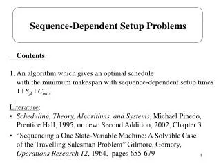
Sequence-Dependent Setup Problems. Contents 1. An algorithm which gives an optimal schedule with the minimum makespan with sequence-dependent setup times 1 | S jk | C max. Literature :

Sequence-Dependent Setup Problems
E N D
Presentation Transcript
Sequence-Dependent Setup Problems Contents 1. An algorithm which gives an optimal schedule with the minimum makespan with sequence-dependent setup times 1 | Sjk | Cmax • Literature: • Scheduling, Theory, Algorithms, and Systems, Michael Pinedo, Prentice Hall, 1995, or new: Second Addition, 2002, Chapter 3. • “Sequencing a One State-Variable Machine: A Solvable Case of the Travelling Salesman Problem” Gilmore, Gomory, Operations Research 12, 1964, pages 655-679
Single machine: rj=0, no sequence dependent setup times • 1 | Sjk | Cmax NP hard • a single real variable which describes each job • job j: to start the job the machine must be in state aj , • at the completion of the job the machine state is bj • sjk = | ak - bj | job k follows job j • Travelling Salesman Problem • with n+1 cities j0, j1, …,jn, j0 • k = (j) travelling salesman leaving city j for city k
{0, 1, 2, 3} {2, 3, 1, 0} (0) = 2 (1) = 3 (2) = 1 (3) = 0 0 2 0 2 3 1 3 1 {0, 1, 2, 3} {2, 1, 3, 0} bk a(j) bj a(k) b2 a(2) a(1) cost of going from 1 to (1) is | a(1) - b1 | b1
Swap I(j,k) applied to a permutation produces another permutation ’: ’(k) = (j) ’(j) = (k) ’(l) = (l), l j , k 5 5 1 1 4 4 2 3 2 3 6 7 6 7 11 11 8 8 10 9 10 9
a(k) bk change in cost due to swap I(j, k) a(j) bj Lemma. If the swap causes two arrows that did nor cross earlier to cross, then the cost of the tour CI(j,k) increases and vice versa. CI(j, k) = || [bj, bk] [a(j), a(k)] || Lemma. Let * be a permutation that ranks a, that is j > k implies a(j) > a(k), then * is optimal with respect to cost.
Gundirected graph where arcs link the jth and (j)th nodes, j=1,…,n. Spanning tree - a minimal set of additional arcs that connect anunconnected graph. 2 2 2 3 3 3 1 1 1 4 5 4 5 4 5 8 8 8 6 6 6 14 14 14 7 7 7 13 13 13 9 9 9 10 16 10 16 10 16 15 15 15 11 12 12 12 11 11
Theorem. Assume that Ghas p components. Let I(j1, k1), …, I(jp-1, kp-1), be the swaps corresponding to the arcs of a spanning tree G.The arcs may be taken in any order. Then the permutation ’ given by ’= I(j1, k1), …, I(jp-1, kp-1) is a tour. Lemma. There is a minimal cost spanning tree for Gthat contains onlyarcs Rj, j+1.
a(3)=11 b3=10 CI(1, 2) = || [1,6] [2,4] || = 2 (4-2) = 4 CI(2, 3) = || [6,10] [4,11] || = 2 (10-6) = 8 b2=6 a(2 )=4 a(1) =2 b1=1 a(3)=11 a(3)=11 b3=10 b3=10 b2=6 b2=6 a(2 )=4 a(2 )=4 a(1) =2 a(1) =2 b1=1 b1=1 I(1, 2) then I(2, 3) CI(2, 3) = || [6,10] [2,11] || = 2 (10-6) = 8 I(2, 3) then I(1, 2) CI(1, 2) = || [1,6] [2,11] || = 2 (6-2) = 8 CHANGED!
A node is of Type 1 if bja(j) (arrow points up) A node is of Type 2 if bj>a(j) (arrow points down) A swap is of Type 1 if lower node is of Type 1 A swap is of Type 2 if lower node is of Type 2 If swaps I(j, j+1) of Type 1 are performed in decreasing order of the node indices, followed by swaps of Type 2 in increasing order of the node indices then a single tour is obtained without changing anyC* I(j, j+1) involved in the swaps
Algorithm + Example 7 jobs Step 1. Arrange the bj in order of size and renumber the jobs so that b1b2 ... bn Arrange the aj in order of size. The permutation mapping *is defined by * (j) = k, k being such that ak is the jth smallest of the a.
a4=45 b7=40 a6=34 b6=31 b5=26 a5=22 b4=19 a7=18 a3=16 b3=15 a1=7 b2=3 a2=4 b1=1
Step 2. Form an undirected graph with n nodes and undirected arcs connecting the jth and *(j) nodes, j=1,…n . If the current graph has only one component then STOP ; otherwise go to Step 3. 2 1 3 7 4 6 5
Step 3. Compute the swap costs C*I(j, j+1) for j=1,…,n C* I(j, j+1) = 2 max ( min (bj+1, a*(j+1)) - max (bj, a*(j)) ), 0 ) C* I(1, 2) = 2 max ( (3-4), 0 ) = 0 C* I(2, 3) = 2 max ( (15-7), 0 ) = 16 C* I(3, 4) = 2 max ( (18-16), 0 ) = 4 C* I(4, 5) = 2 max ( (22-19), 0 ) = 6 C* I(5, 6) = 2 max ( (31-26), 0 ) = 10 C* I(6, 7) = 2 max ( (40-34), 0 ) = 12
2 16 1 3 4 7 4 6 6 10 5 Step 4. Select the smallest value C* I(j, j+1) such that j is in one componentand j+1 in another. In case of a tie for smallest, choose any. Insert the undirected arc Rj, j+1 into the graph. Repeat this step untilall the components in the undirected graph are connected. 2 2 2 1 1 1 3 3 3 4 4 4 7 7 7 4 4 4 6 6 6 6 6 5 5 10 5
Step 5. Divide the arcs added in Step 4 into two groups. Those Rj, j+1 for which bja(j) go in group 1, those for which bj>a(j) go in group 2. Step 6. Find the largest index j1 such that Rj1, j1+1 is in group 1. Find the second largest index, and so on, up to jl assuming there arel elements in the group. Find the smallest index k1 such that Rk1, k1+1 is in group 2. Find the second smallest index, and so on, up to km assuming there arem elements in the group. j1 = 3, j2 = 2, k1 = 4, k2 = 5
Step 7. The optimal tour ** is constructed by applying the followingsequence of swaps on the permutation *: ** = * I(j1,j1+1) I(j2,j2+1) … I(jl,jl+1) I(k1,k1+1) I(k2, k2+1) … I(km,km+1) ** = * I(3,4) I(2,3) I(4,5) I(5,6) Type 1 Type 2
a4=45 a4=45 b7=40 b7=40 a6=34 a6=34 b6=31 b6=31 b5=26 b5=26 a5=22 a5=22 b4=19 a7=18 b4=19 a7=18 a3=16 a3=16 b3=15 b3=15 a1=7 a1=7 b2=3 a2=4 b2=3 a2=4 b1=1 b1=1 * I(3,4) I(2,3) * I(3,4)
a4=45 a4=45 b7=40 b7=40 a6=34 a6=34 b6=31 b6=31 b5=26 b5=26 a5=22 a5=22 b4=19 a7=18 b4=19 a7=18 a3=16 a3=16 b3=15 b3=15 a1=7 a1=7 b2=3 a2=4 b2=3 a2=4 b1=1 b1=1 * I(3,4) I(2,3) I(4,5) ** = * I(3,4) I(2,3) I(4,5) I(5,6)
a4=45 b7=40 a6=34 b6=31 b5=26 a5=22 b4=19 a7=18 a3=16 b3=15 a1=7 b2=3 a2=4 b1=1 ** = * I(3,4) I(2,3) I(4,5) I(5,6) The optimal tour is: 1 2 7 4 5 6 3 1 The cost of the tour is: 3 + 15 + 5 + 3 + 8 + 15 + 8 = 57
Summary • 1 | Sjk | Cmax , sjk = | ak - bj | a polynomial time algorithm is given • 1 | Sjk | Cmax is NP hard