Download
1 / 26
280 likes | 525 Vues
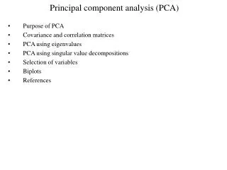
an introduction to Principal Component Analysis (PCA). abstract. Principal component analysis (PCA) is a technique that is useful for the compression and classification of data. The purpose is to reduce the dimensionality of a data set (sample) by finding a new set of variables,

E N D
an introduction to Principal Component Analysis (PCA)
abstract Principal component analysis (PCA) is a technique that is useful for the compression and classification of data. The purpose is to reduce the dimensionality of a data set (sample) by finding a new set of variables, smaller than the original set of variables, that nonetheless retains most of the sample's information. By information we mean the variation present in the sample, given by the correlations between the original variables. The new variables, called principal components (PCs), are uncorrelated, and are ordered by the fraction of the total information each retains.
overview • geometric picture of PCs • algebraic definition and derivation of PCs • usage of PCA • astronomical application
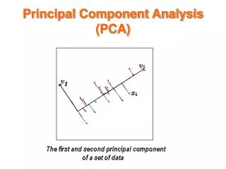
Geometric picture of principal components (PCs) A sample of n observations in the 2-D space Goal: to account for the variation in a sample in as few variables as possible, to some accuracy
Geometric picture of principal components (PCs) • the 1st PC is a minimum distance fit to a line in space • the 2nd PC is a minimum distance fit to a line • in the plane perpendicular to the 1st PC PCs are a series of linear least squares fits to a sample, each orthogonal to all the previous.
Algebraic definition of PCs Given a sample of n observations on a vector of p variables define the first principal component of the sample by the linear transformation λ where the vector is chosen such that is maximum
Algebraic definition of PCs Likewise, define the kth PC of the sample by the linear transformation λ where the vector is chosen such that is maximum subject to and to
Algebraic derivation of coefficient vectors To find first note that where is the covariance matrix for the variables
Algebraic derivation of coefficient vectors To find maximize subject to Let λ be a Lagrange multiplier then maximize by differentiating… therefore is an eigenvector of corresponding toeigenvalue
Algebraic derivation of We have maximized So is the largest eigenvalue of The first PC retains the greatest amount of variation in the sample.
Algebraic derivation of coefficient vectors To find the next coefficient vector maximize subject to and to First note that then let λ and φ be Lagrange multipliers, and maximize
Algebraic derivation of coefficient vectors We find that is also an eigenvector of whose eigenvalue is the second largest. In general • The kth largest eigenvalue of is the variance of the kth PC. • The kth PC retains the kth greatest fraction • of the variation in the sample.
Algebraic formulation of PCA Given a sample of n observations on a vector of p variables define a vector of p PCs according to where is an orthogonal pxp matrix whose kth column is the kth eigenvector of Then is the covariance matrix of the PCs, being diagonal with elements
usage of PCA: Probability distribution for sample PCs If (i) the n observations of in the sample are independent & • is drawn from an underlying population that • follows a p-variate normal (Gaussian) distribution • with known covariance matrix then where is the Wishart distribution else utilize a bootstrap approximation
usage of PCA: Probability distribution for sample PCs If (i) follows a Wishart distribution & • the population eigenvalues are all distinct then the following results hold as • all the are independent of all the • and are jointly normally distributed (a tilde denotes a population quantity)
usage of PCA: Probability distribution for sample PCs and (a tilde denotes a population quantity)
usage of PCA: Inference about population PCs If follows a p-variate normal distribution then analytic expressions exist* for MLE’s of , , and confidence intervals for and hypothesis testing for and else bootstrap and jackknife approximations exist *see references, esp. Jolliffe
usage of PCA: Practical computation of PCs In general it is useful to define standardized variables by If the are each measured about their sample mean then the covariance matrix of will be equal to the correlation matrix of and the PCs will be dimensionless
usage of PCA: Practical computation of PCs Given a sample of n observations on a vector of p variables (each measured about its sample mean) compute the covariance matrix where is the nxp matrix whose ith row is the ith obsv. Then compute the nxp matrix whose ith row is the PC score for the ith observation.
usage of PCA: Practical computation of PCs Write to decompose each observation into PCs
usage of PCA: Data compression Because the kth PC retains the kth greatest fraction of the variation we can approximate each observation by truncating the sum at the first m < p PCs
usage of PCA: Data compression Reduce the dimensionality of the data from p to m < p by approximating where is the nxm portion of and is the pxm portion of
astronomical application: PCs for elliptical galaxies Rotating to PC in BT – Σ space improves Faber-Jackson relation as a distance indicator Dressler, et al. 1987
astronomical application: Eigenspectra (KL transform) Connolly, et al. 1995
references Connolly, and Szalay, et al., “Spectral Classification of Galaxies: An Orthogonal Approach”, AJ, 110, 1071-1082, 1995. Dressler, et al., “Spectroscopy and Photometry of Elliptical Galaxies. I. A New Distance Estimator”, ApJ, 313, 42-58, 1987. Efstathiou, G., and Fall, S.M., “Multivariate analysis of elliptical galaxies”, MNRAS, 206, 453-464, 1984. Johnston, D.E., et al., “SDSS J0903+5028: A New Gravitational Lens”, AJ, 126, 2281-2290, 2003. Jolliffe, Ian T., 2002, Principal Component Analysis (Springer-Verlag New York, Secaucus, NJ). Lupton, R., 1993, Statistics In Theory and Practice (Princeton University Press, Princeton, NJ). Murtagh, F., and Heck, A., Multivariate Data Analysis (D. Reidel Publishing Company, Dordrecht, Holland). Yip, C.W., and Szalay, A.S., et al., “Distributions of Galaxy Spectral Types in the SDSS”, AJ, 128, 585-609, 2004.