Statistical Multiplexing and Link Scheduling
This presentation delves into the intricacies of statistical multiplexing and link scheduling in packet-switched networks. We explore the effects of fixed-capacity links and variable delay due to buffering, as well as the critical role of scheduling algorithms like First-In-First-Out (FIFO), Static Priority (SP), and Earliest Deadline First (EDF). The discussion includes the concept of burstiness and traffic shaping, particularly the token bucket model. We will analyze how maximum flows with delay requirements can be managed effectively in a buffered link environment, providing insights into the benefits and drawbacks of various scheduling strategies.


Statistical Multiplexing and Link Scheduling
E N D
Presentation Transcript
Packet Switch • Fixed-capacity links • Variable delay due to waiting time in buffers • Delay depends on • Traffic • Scheduling
Traffic Arrivals Peak rate Frame size Mean rate Frame number
First-In-First-Out (FIFO) • Packets are transmitted in the order of their arrivals • FIFO is the default scheduling in packet networks • Main Drawbacks of FIFO: • Unfairness in overload: Traffic with most arrivals receives most of the bandwdith • Unable to differentiate traffic with different requirements
Static Priority (SP) • Blind Multiplexing (BMux): All “other traffic” has higher priority
Earliest Deadline First (EDF) Benchmark scheduling algorithm for meeting delay requirements
Disclaimer • This talk makes a few simplifications
Traffic Description • Traffic arrivals in time interval [s,t) is • Burstiness can be reduced by “shaping” traffic Cumulative arrivals A
Shaped Arrivals Flow 1 . . . C Flow N Flows areshaped Buffered Link Regulated arrivals Traffic is shaped by an envelope such that: Popular envelope: “token bucket”
What is the maximum number of shaped flows with delay requirements that can be put on a single buffered link? • Link capacity C • Each flows j has • arrival function Aj • envelope Ej • delay requirement dj
Delay Analysis of Schedulers • Consider a link scheduler with rate C • Consider arrival from flow i at t with t+di: Arrivals from flow j Deadline of Tagged arrival Tagged arrival Limit (Scheduler Dependent) • Tagged arrival departs by if
Delay Analysis of Schedulers Arrivals from flow j • with • FIFO: • Static Priority: • EDF:
Schedulability Condition We have: Therefore: An arrival from class i never has a delay bound violation if Condition is tight, when Ej is concave
Numerical Result (Sigmetrics 1995) C = 45 Mbps MPEG 1 traces: Lecture: d = 30 msec Movie (Jurassic Park): d = 50 msec EDF Static Priority (SP) Peak Rate strong effective envelopes Type 1 flows
Expected case Probable worst-case Deterministic worst-case
Worst-casebacklog Backlog Backlog Statistical Multiplexing Gain Worst-case arrivals Arrivals Flow 1 Flow 2 Flow 3 Time With statistical multiplexing Arrivals Flow 1 Flow 2 Flow 3 Time Backlog
Statistical Multiplexing Gain Statistical multiplexing gain is the raison d’être for packet networks.
What is the maximum number of flows with delay requirements that can be put on a buffered link and considering statistical multiplexing? • Arrivalsare random processes • Stationarity: is stationary random processes • Independence: Any two flows and are stochastically independent
Envelopes for random arrivals Statistical envelope bounds arrival from flow j with high certainty • Statistical envelope : Statistical envelopes are non-random functions
Arrivals from group of flows: with deterministic envelopes: with statistical envelopes: Aggregating arrivals
Statistical envelope for group of indepenent (shaped) flows • Exploit independence and extract statistical multiplexing gain when calculating • For example, using the Chernoff Bound, we can obtain
Statistical vs. Deterministic Envelope Envelopes (JSAC 2000) statistical envelopes Type 1 flows: P =1.5 Mbps r = .15 Mbps s =95400 bits Type 2 flows: P = 6 Mbps r = .15 Mbps s = 10345 bits Type 1 flows
Statistical vs. Deterministic Envelope Envelopes (JSAC 2000) statistical envelopes Type 1 flows: P =1.5 Mbps r = .15 Mbps s =95400 bits Type 2 flows: P = 6 Mbps r = .15 Mbps s = 10345 bits Type 2 flows
Statistical vs. Deterministic Envelope Envelopes (JSAC 2000) Traffic rate at t = 50 msType 1 flows
Deterministic Service Never a delay bound violation if: Scheduling Algorithms • Work-conserving scheduler that serves Q classes • Class-q has delay bound dq • D-scheduling algorithm . . . Scheduler Statistical Service Delay bound violation with if:
Statistical multiplexing makes a big difference Scheduling has small impact Statistical Multiplexing vs. Scheduling (JSAC 2000) Example: MPEG videos with delay constraints at C= 622 Mbps Deterministic service vs. statistical service (e = 10-6) dterminator=100 ms dlamb=10 ms Thick lines: EDF SchedulingDashed lines: SP scheduling
Peak rate effectivebandwidth Mean rate More interesting traffic types • So far: Traffic of each flow was shaped • Next: • On-Off traffic • Fraction Brownian Motion (FBM) traffic Approach: • Exploit literature on Effective Bandwidth • Derived for many traffic types
Statistical Envelopes and Effective Bandwidth Effective Bandwidth (Kelly 1996) Given , an effective envelope is given by
Different Traffic Types (ToN 2007) Comparisons of statistical service guarantees for different schedulers and traffic types Schedulers: SP- Static PriorityEDF – Earliest Deadline FirstGPS – Generalized Processor Sharing Traffic: Regulated – leaky bucketOn-Off – On-off sourceFBM – Fractional Brownian Motion C= 100 Mbps, e = 10-6
Delays on a path with multiple nodes: • Impact of Statistical Multiplexing • Role of Scheduling • How do delays scale with path length? • Does scheduling still matter in a large network?
Back to scheduling … So far: Through traffic has lowest priority and gets leftover capacity Leftover Service or Blind Multiplexing BMux C How do end-to-end delay bounds look like for different schedulers? Does link scheduling matter on long paths?
Service curves vs. schedulers (JSAC 2011) • How well can a service curve describe a scheduler? • For schedulers considered earlier, the following is ideal: with indicator function and parameter
Example: End-to-End Bounds • Traffic is Markov Modulated On-Off Traffic (EBB model) • Fixed capacity link
Example: Deterministic E2E Delays • C = 100 Mbps • Peak rate: P = 1.5 MbpsAverage rate: r = 0.15 Mbps BMUX EDF(delay-tolerant) FIFO EDF(delay intolerant
Example: Statistical E2E Delays • C = 100 Mbps • e = 10-9 • Peak rate: P = 1.5 MbpsAverage rate: r = 0.15 Mbps