Complex Data
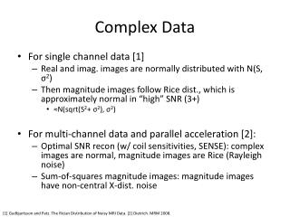
Complex Data. For single channel data [1] Real and imag . images are normally distributed with N(S, σ 2 ) Then magnitude images follow Rice dist., which is approximately normal in “high” SNR (3+) ≈N( sqrt (S 2 + σ 2 ), σ 2 ) For multi-channel data and parallel acceleration [2]:

Complex Data
E N D
Presentation Transcript
Complex Data • For single channel data [1] • Real and imag. images are normally distributed with N(S, σ2) • Then magnitude images follow Rice dist., which is approximately normal in “high” SNR (3+) • ≈N(sqrt(S2+ σ2), σ2) • For multi-channel data and parallel acceleration [2]: • Optimal SNR recon (w/ coil sensitivities, SENSE): complex images are normal, magnitude images are Rice (Rayleigh noise) • Sum-of-squares magnitude images: magnitude images have non-central Χ-dist. noise [1] Gudbjartsson and Patz. The Rician Distribution of Noisy MRI Data. [2] Dietrich. MRM 2008.
CRLB with Complex Data • In previous designs, the algorithm was allowed to optimize σi2 for each magnitude image with Σσi2= constant • For the complex data case, the real and imag. images are assumed to have same noise level • Thus the situation is essentially the same, where we choose σi2 for each series • Further, the results should be comparable to previous ones with magnitude images • Due to the relations in noise variance between complex and magnitude images, i.e. for reasonable SNR, the variances are all about the same
B0 Robustness • Previously, a question about how finely to sample the off-resonance phase for the design • This is plotted with 100 points • I use 64 points in the analysis • Now takes 2+ days to solve all the problems up to 16 total images
Optimal Design • The Li paper used a criterion as σ/θ2, a greater scaling than CoV citing [3] • Still need go through that to understand why that’s a logical/better choice • “Alphabetic” optimality of Fisher information matrix • A-optimality –minimize the mean of CRLBs, tr(F-1) • D-optimality – minimize the determinant, |F-1| • E-optimality – maximize the smallest eigenvalue of F • Previously you may remember we looked at the SVD of J for mcDESPOT • G-optimality – minimize the maximum variance of a parameter • We’re doing a weighted combination (by 1/θ) version of A • Often times these variants have the same optimal design • They each have different properties and perhaps some are easier to solve, need to read more [3] Atkinson, Donev, and Tobias. Optimal Experimental Designs.
Thoughts • Is complex data worth pursuing? • Definitely a big improvement over magn. only, which seemed terrible • But is it improved enough? • Should evaluate DESPOT2-FM for comparison • I might expect it to not do that great as I had tough time with it for mouse data • Other study data had much less severe B0 inhomogeneity