Quantum Mechanical Cross Sections: Understanding Scattering in Quantum Systems
180 likes | 319 Vues
This article discusses the foundational principles of quantum mechanical cross sections, starting with initial and final states of a target and projectile. It explores the time evolution governed by the Hamiltonian, as defined in quantum mechanics through the Schrödinger equation. The role of the S-matrix in predicting transitions, particle decay rates, and the calculation of differential cross sections in scattering experiments are highlighted. The interplay between free Hamiltonians and interaction terms establishes a framework for understanding how quantum systems evolve and interact.

Quantum Mechanical Cross Sections: Understanding Scattering in Quantum Systems
E N D
Presentation Transcript
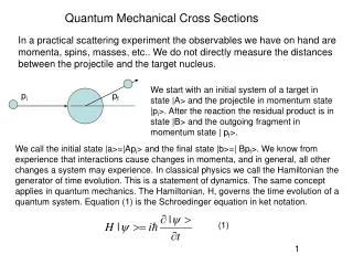
Quantum Mechanical Cross Sections We start with an initial system of a target in state |A> and the projectile in momentum state |pi>. After the reaction the residual product is in state |B> and the outgoing fragment in momentum state | pf>. pi pf In a practical scattering experiment the observables we have on hand are momenta, spins, masses, etc.. We do not directly measure the distances between the projectile and the target nucleus. We call the initial state |a>=|Api> and the final state |b>=| Bpf>. We know from experience that interactions cause changes in momenta, and in general, all other changes a system may experience. In classical physics we call the Hamiltonian the generator of time evolution. This is a statement of dynamics. The same concept applies in quantum mechanics. The Hamiltonian, H, governs the time evolution of a quantum system. Equation (1) is the Schroedinger equation in ket notation. (1) 1
We define the time evolution operator U(t,t0) such that a system evolves from some initial configuration, |a> to a final configuration |c> according to |c; t> = U(t,t0) |a; t0>. U(t,t0) is a function of the Hamiltonian. The relationship between U(t,t0) and the Hamiltonian is worked out in books on quantum mechanics (ref. 1,2). We will assume that the target and projectile have some internal Hamiltonians HA and Hp and that the target and projectile interact via an interaction V. The total Hamiltonian is H = HA + Hp + V = H0 + V. Where H0 = HA + Hp , is called the free Hamiltonian. We assume that V becomes negligibly small for large separations between the projectile and target. The total time evolution operator can be written as ( ref.2) U(t,t0) = U0(t,t0) UI(t,t0) . In this expression U0(t,t0) is the time evolution operator derived from the free Hamiltonian and UI(t,t0) depends on both H0 and V. It is expressed in the integral equation 2
We assume that the free Hamiltonian is time independent. Then U0(t’,t0) in equation (4) is the time evolution operator due to H0. If the states |a> and |b> are eigenstates of H0, then the time evolved states of |a> and |b> are The time evolved state |c; t> = U(t,t0) |a; t0> is given by ( ref. 2), Equation (6) tells us that at time t=-T/2 the system is initially in state |a>. At time T/2 the system has evolved into state |c;T/2> which consists of a sum of possible eigenstates |b;-T/2>, each weighted with an amplitude given by Sba , which is time dependent. If we let T/2 and –T/2 go to infinity, then Sba is called the “S – matrix”. The S-matrix must be properly normalized (See ref. 2 chapt. 3). Particle decay rates and cross sections can be calculated once the S-matrix is known. 3
From our discussion in lecture 2 we determined that the scattering rate is We want to connect this derivation to a quantum calculation. The probability that the initial state a will make the transition to b is | Sba|2 . If N t is the number of targets in the box of sides L, and DNp the number of projectiles which have traversed the box then the number of transitions from state a to b is : L L L 4
In an actual calculation the S-matrix will contain terms that cancel the L3 term in (7). In a non-relativistic calculation v = p/m, whereas for the relativistic case v = p/E. Examples of the differential cross section Ds are: Elastic scattering of a particle into a solid angle DW. Projectile scattering into a solid angle DW, and momentum bite Dp. Cross section for 3 body final state, as in 3He(e,e’p)2H, ( 2 bound nuclear states) 5
Multi-body final state where the electron and proton are detected, in 3He(e,e’p)X , Examples of calculating the S-matrix ( ref. 2 chapter 3). We want to calculate since From eqn(6) 6
The states are assumed to be orthonormal so we get Substituting eqn (2) into eqn (8) yields Equation (9) implicitly includes the time evolution operator, so solutions to (9) are obtained through successive iterations, for example, If we substitute this expression into eqn (9) we obtain 7
Eqn (10) is the first approximation, or Born approximation, in the perturbation series expansion of the S-matrix. The expansion can be carried out to higher orders as can be seen. The second order term in the expansion is We will focus on the first term, equation (10), as an approximation for the S-matrix. 8
From equation (3) we obtain HI. Consider the case where the interaction V is time independent. Then the time integral only includes the exponential term. As we let T go to infinity the time integral becomes a delta function in energy. However, we will take the limit of T to infinity a bit later in the calculation. 9
Substituting (12) into (7) we get for the differential cross section, 10
We now take advantage of eqn 5.6.31 in ref. 1, And we obtain for the cross section We see that conservation of energy automatically appears if the time interval T is long enough. We will use (13) to calculate the quantum mechanical cross section in the first approximation (Born approximation) of the S-matrix. Note that the matrix element is, 11
Cross section for potential scattering In a practical scattering situation we have a finite acceptance for a detector with a solid angle DW. There is a range of momenta which are allowed by kinematics which can contribute to the cross section. The cross section for scattering into DW is then obtained as an integral over all the allowed momenta for that solid angle. In the case of potential scattering we will assume only elastic scattering is allowed. This means that there is a change in momentum between the incoming particle and outgoing particle. We are using periodic boundary conditions, or box normalization, ( see ref. 2) for which the incoming and outgoing states are plane wave states. The incoming wave |a> is 12
The outgoing state |b> is All possible outgoing states |b> which can be accepted by the solid angle must be included in the summation. We next substitute the matrix element into the above equation. This will be an integral over all relevant degrees of freedom needed to describe the states a and b. For a position dependent interaction and the plane waves above, the integration is over configuration space. 13
But we will consider only potentials diagonal ( local) in configuration space. Notice that the matrix element is proportional to the Fourier transform of the potential. q 14
In eqn (17) we note the sum over possible n values. The smallest change possible in n is dn = 1. We want to convert the sum in (17) into an integral over wave numbers. And from eqns (15) we realize that 15
We substitute (18) into (17) an obtain Note that in the delta function in (20) we have functions ( the energies) of the momenta k, whereas the variable of integration is k. We use the following property of functions of the delta function. In the case of potential scattering, or elastic scattering, the zeroes occur for k = kb = ka . The derivative of the energy with respect to the wave number k is 16
Integrating over k, the delta function selects the value k = ka which we will simply call k, the magnitude of the initial wave number. Thus, We are now in a position to evaluate the differential elastic cross section using eqn (21) for any potential V. We will need to find the Fourier transform of the potential as a function of q. 17
(1) “Modern Quantum Mechanics – Revised Edition”, J. J. Sakurai, Addison-Wesley, 1994 (2) “Relativistic Quantum Mechanics and Field Theory”, Franz Gross, John Wiley & Sons, 1993 18