Download
1 / 36
370 likes | 590 Vues
Statistical Analysis of Canopy Turbulence. Problem: Linking Measurements to Fluid Dynamics Equations. Turbulence is a stochastic phenomena Comparing measurements (e.g. time series) and model predictions can only be conducted statistically.

E N D
Problem: Linking Measurements to Fluid Dynamics Equations • Turbulence is a stochastic phenomena • Comparing measurements (e.g. time series) and model predictions can only be conducted statistically. • What are the appropriate assumptions in such comparisons in field experiments?
Outline • Introduction: Linking eddy-sizes, averaging operations through the ergodic hypothesis. • Idealized setup: Model canopy in a flume as a case study to highlight the relevant eddy-sizes and the spatial-temporal averaging. • Real-world setup: Stable flows near the canopy-atmosphere interface. No unique canonical form for the integral length - but several possible canonical forms are examined depending on “external boundary conditions” and “inherent” length scales. • Conclusions:
Introduction • Three types of averaging: Spatial, Temporal, and Ensemble. • Averaging equations of motion: proper averaging operator is ensemble. • Field experiments - typically provide temporal averaging. • Key assumption when linking equations to measurements: Ergodic hypothesis
Poor-Man’s version of the Navier-Stokes Equation Why Ensemble-Averaging is the appropriate operator? Analogy borrowed from Frisch (1995)
Introduction:Averaging • Monin and Yaglom (1971): u(t) Experiment Number
Weakly Stationary Process: • Ensemble Mean independent of time • Ensemble Variance independent of time • Ensemble covariance - only dependent on time lag Note: Ensemble averaging is referred to as E
E(u) or E(u2) t Ergodic Hypothesis: T E [u,u(t+ ) ] For stationary process: Ensemble average = time average If :1) Ensemble Autocovariance decays as 2) Individual Autocovariance decays as
Sampling Period and Eddy-sizes A weaker version of these conditions: Integral time scale of one realization is finite: ~ Energetic Scale Lumley and Panofsky (1964): T>>
LIDAR EXPERIMENTS LIDAR Sight Lidar Experiments at UC Davis - 1991 Ground (Bare Soil) 3m LIDAR
ERGODIC HYPOTHESIS FOR CANOPY TURBULENCE • ASL: Ergodic hypothesis seems reasonable. • CSL: Two types of averaging are employed - spatial and temporal. What are the canonical length scales and how they affect both averaging operations.
FLUME EXPERIMENTS: • To understand the connection between energetic length scales, spatial and temporal averaging, start with an idealized canopy (Finnigan, 2000). • Vertical rods within a flume. • Repeat the experiment for 5 canopy densities (sparse to dense) and 2 Re
Test section Flow direction Open channel FLUME DIMENSIONS 1 m • PLAN 9 m 1m
Rods positions Weighted scheme 2 cm hw h dr Canopy sublayer 2h 1 cm FLUME EXPERIMENTS • PLAN • VIEW + + +++++++ + + ++++ SECTION VIEW
REGION III REGION II d Displaced wall REGION I Real wall Canonical Form of the CSL THE FLOW FIELD IS A SUPERPOSITION OF THREE CANONICAL STRUCTURES Mixing Layer Boundary Layer
Structure of Turbulence in Model Plant Canopy • Lowest Layers in the Canopy: Flow Visualizations Laser Sheet
Flow Visualization • Flow visualization supports the hypothesis that the structure of turbulence in the deeper layers of the canopy is dominated by Von Karman streets periodically interrupted by sweep events from the top layers.
Von Karman Streets NASA’s EOS MODIS Von Karman streets shedding off the Cape Verde Islands
The flow field is dominated by small vorticity generated by von Kàrmàn vortex streets. Strouhal Number = f d / u = 0.21 (independent of Re) REGION I: FLOW DEEP WITHIN THE CANOPY Spectra of w
REGION II: Combine Mixing Layer and Boundary Layer Re1 • LBL= Boundary Layer Length = k(z-d) • LML = Mixing Layer Length = Shear Length Scale • l = Total Mixing Length Estimated from an eddy-diffusivity Re2
Spatial Averaging and Dispersive Fluxes: Consistent with: 1) Bohm et al. (2000) 2) Cheng and Castro (2002) • Dispersive Fluxes = Roughness Density Roughness Density a a % % Roughness Density
CSL Flows in Complex Morphology and Stability CSL flows for simple morphology and canopy density does have well-defined length and time scales (~Ergodic). CSL flows for stable conditions in real canopies??
cospectrum quad-spectrum coherence phase Ramps: Cross-spectra
cospectrum quad-spectrum coherence phase Ramps: Cross-spectra
Gravity Waves: Stable Boundary Layer at z/h = 1.12 (Duke Forest)
cospectrum quad-spectrum coherence phase Gravity Waves: Cross-spectra
cospectrum quad-spectrum coherence phase Gravity Waves: Cross-spectra
Autocorrelation function of temperature Gravity waves Ramps t = 12 sec t = 30 sec Time lag Time lag t = 20 sec Net Radiation Time lag
Well-Developed Turbulence No Turbulence Slightly Stable Flows Gravity Waves Ramps Two End-members of stable CSL State
Conclusions: • For ASL flows over uniform surfaces, the ergodic hypothesis is reasonable. • For neutral flows within the CSL of simple morphology, the ergodic hypothesis is also reasonable. • For stable CSL flows, too much “contamination” from boundary conditions (e.g. clouds or other disturbances) to sustain stationarity.