Lecture 15 Multimedia Instruction Sets: SIMD and Vector
560 likes | 577 Vues
Explore the significance of SIMD and vector instructions in multimedia processing, discussing the need for specialized ISAs, characteristics of multimedia applications, and examples of media functions. Learn about SIMD extensions for general-purpose processors and programming approaches for maximizing performance.

Lecture 15 Multimedia Instruction Sets: SIMD and Vector
E N D
Presentation Transcript
Lecture 15Multimedia Instruction Sets:SIMD and Vector Christoforos E. Kozyrakis (kozyraki@cs.berkeley.edu) CS252 Graduate Computer Architecture University of California at Berkeley March 14th, 2001
What is Multimedia Processing? • Desktop: • 3D graphics (games) • Speech recognition (voice input) • Video/audio decoding (mpeg-mp3 playback) • Servers: • Video/audio encoding (video servers, IP telephony) • Digital libraries and media mining (video servers) • Computer animation, 3D modeling & rendering (movies) • Embedded: • 3D graphics (game consoles) • Video/audio decoding & encoding (set top boxes) • Image processing (digital cameras) • Signal processing (cellular phones)
The Need for Multimedia ISAs • Why aren’t general-purpose processors and ISAs sufficient for multimedia (despite Moore’s law)? • Performance • A 1.2GHz Athlon can do MPEG-4 encoding at 6.4fps • One 384Kbps W-CDMA channel requires 6.9 GOPS • Power consumption • A 1.2GHz Athlon consumes ~60W • Power consumption increases with clock frequency and complexity • Cost • A 1.2GHz Athlon costs ~$62 to manufacture and has a list price of ~$600 (module) • Cost increases with complexity, area, transistor count, power, etc
Parsing Dequantization IDCT RGB->YUV Example: MPEG Decoding Input Stream Load Breakdown 10% 20% 25% Block Reconstruction 30% 15% Output to Screen
Example: 3D Graphics Display Lists Load Breakdown Transform Lighting Geometry Pipe 10% 10% Setup Rasterization Anti-aliasing Shading, fogging Texture mapping Alpha blending Z-buffer Clipping Frame-buffer ops 35% Rendering Pipe 55% Output to Screen
Characteristics of Multimedia Apps (1) • Requirement for real-time response • “Incorrect” result often preferred to slow result • Unpredictability can be bad (e.g. dynamic execution) • Narrow data-types • Typical width of data in memory: 8 to 16 bits • Typical width of data during computation: 16 to 32 bits • 64-bit data types rarely needed • Fixed-point arithmetic often replaces floating-point • Fine-grain (data) parallelism • Identical operation applied on streams of input data • Branches have high predictability • High instruction locality in small loops or kernels
Characteristics of Multimedia Apps (2) • Coarse-grain parallelism • Most apps organized as a pipeline of functions • Multiple threads of execution can be used • Memory requirements • High bandwidth requirements but can tolerate high latency • High spatial locality (predictable pattern) but low temporal locality • Cache bypassing and prefetching can be crucial
Matrix transpose/multiply DCT/FFT Motion estimation Gamma correction Haar transform Median filter Separable convolution Viterbi decode Bit packing Galois-fields arithmetic … (3D graphics) (Video, audio, communications) (Video) (3D graphics) (Media mining) (Image processing) (Image processing) (Communications, speech) (Communications, cryptography) (Communications, cryptography) Examples of Media Functions
Approaches to Mediaprocessing General-purpose processors with SIMD extensions Vector Processors VLIW with SIMD extensions (aka mediaprocessors) Multimedia Processing DSPs ASICs/FPGAs
SIMD Extensions for GPP • Motivation • Low media-processing performance of GPPs • Cost and lack of flexibility of specialized ASICs for graphics/video • Underutilized datapaths and registers • Basic idea: sub-word parallelism • Treat a 64-bit register as a vector of 2 32-bit or 4 16-bit or 8 8-bit values (short vectors) • Partition 64-bit datapaths to handle multiple narrow operations in parallel • Initial constraints • No additional architecture state (registers) • No additional exceptions • Minimum area overhead
* * * * + + Example of SIMD Operation (1) Sum of Partial Products
Example of SIMD Operation (2) Pack (Int16->Int8)
Summary of SIMD Operations (1) • Integer arithmetic • Addition and subtraction with saturation • Fixed-point rounding modes for multiply and shift • Sum of absolute differences • Multiply-add, multiplication with reduction • Min, max • Floating-point arithmetic • Packed floating-point operations • Square root, reciprocal • Exception masks • Data communication • Merge, insert, extract • Pack, unpack (width conversion) • Permute, shuffle
Summary of SIMD Operations (2) • Comparisons • Integer and FP packed comparison • Compare absolute values • Element masks and bit vectors • Memory • No new load-store instructions for short vector • No support for strides or indexing • Short vectors handled with 64b load and store instructions • Pack, unpack, shift, rotate, shuffle to handle alignment of narrow data-types within a wider one • Prefetch instructions for utilizing temporal locality
Programming with SIMD Extensions • Optimized shared libraries • Written in assembly, distributed by vendor • Need well defined API for data format and use • Language macros for variables and operations • C/C++ wrappers for short vector variables and function calls • Allows instruction scheduling and register allocation optimizations for specific processors • Lack of portability, non standard • Compilers for SIMD extensions • No commercially available compiler so far • Problems • Language support for expressing fixed-point arithmetic and SIMD parallelism • Complicated model for loading/storing vectors • Frequent updates • Assembly coding
SIMD Performance Limitations • Memory bandwidth • Overhead of handling alignment and data width adjustments
A Closer Look at MMX/SSE • Higher speedup for kernels with narrow data where 128b SSE instructions can be used • Lower speedup for those with irregular or strided accesses
CS 252 Administrivia • No announcements for today • Chip design “toys” to see during break • Wafers • Packages • Packaged chips • Boards
VECTOR (N operations) SCALAR (1 operation) v2 v1 r2 r1 + + r3 v3 vector length add r3, r1, r2 vadd.vv v3, v1, v2 Vector Processors • Initially developed for super-computing applications, but we will focus only on multimedia today • Vector processors have high-level operations that work on linear arrays of numbers: "vectors"
Properties of Vector Processors • Single vector instruction implies lots of work (loop) • Fewer instruction fetches • Each result independent of previous result • Compiler ensures no dependencies • Multiple operations can be executed in parallel • Simpler design, high clock rate • Reduces branches and branch problems in pipelines • Vector instructions access memory with known pattern • Effective prefetching • Amortize memory latency of over large number of elements • Can exploit a high bandwidth memory system • No (data) caches required!
Styles of Vector Architectures • Memory-memory vector processors • All vector operations are memory to memory • Vector-register processors • All vector operations between vector registers (except vector load and store) • Vector equivalent of load-store architectures • Includes all vector machines since late 1980s • We assume vector-register for rest of the lecture
Components of a Vector Processor • Scalar CPU: registers, datapaths, instruction fetch logic • Vector register • Fixed length memory bank holding a single vector • Has at least 2 read and 1 write ports • Typically 8-32 vector registers, each holding 1 to 8 Kbits • Can be viewed as array of 64b, 32b, 16b, or 8b elements • Vector functional units (FUs) • Fully pipelined, start new operation every clock • Typically 2 to 8 FUs: integer and FP • Multiple datapaths (pipelines) used for each unit to process multiple elements per cycle • Vector load-store units (LSUs) • Fully pipelined unit to load or store a vector • Multiple elements fetched/stored per cycle • May have multiple LSUs • Cross-bar to connect FUs , LSUs, registers
Basic Vector Instructions Instr. OperandsOperationComment VADD.VVV1,V2,V3 V1=V2+V3 vector + vector VADD.SVV1,R0,V2 V1=R0+V2 scalar + vector VMUL.VV V1,V2,V3 V1=V2xV3 vector x vector VMUL.SV V1,R0,V2 V1=R0xV2 scalar x vector VLD V1,R1 V1=M[R1..R1+63] load, stride=1 VLDS V1,R1,R2 V1=M[R1..R1+63*R2] load, stride=R2 VLDX V1,R1,V2 V1=M[R1+V2i,i=0..63] indexed("gather") VST V1,R1 M[R1..R1+63]=V1 store, stride=1 VSTS V1,R1,R2 V1=M[R1..R1+63*R2] store, stride=R2 VSTX V1,R1,V2 V1=M[R1+V2i,i=0..63] indexed(“scatter") + all the regular scalar instructions (RISC style)…
Vector Memory Operations • Load/store operations move groups of data between registers and memory • Three types of addressing • Unit stride • Fastest • Non-unit(constant) stride • Indexed (gather-scatter) • Vector equivalent of register indirect • Good for sparse arrays of data • Increases number of programs that vectorize • Support for various combinations of data widths in memory and registers • {.L,.W,.H.,.B} x {64b, 32b, 16b, 8b}
64 element SAXPY: scalar LD R0,a ADDI R4,Rx,#512 loop: LD R2, 0(Rx) MULTD R2,R0,R2 LD R4, 0(Ry) ADDD R4,R2,R4 SD R4, 0(Ry) ADDI Rx,Rx,#8 ADDI Ry,Ry,#8 SUB R20,R4,Rx BNZ R20,loop 64 element SAXPY: vector LD R0,a #load scalar a VLD V1,Rx #load vector X VMUL.SV V2,R0,V1 #vector mult VLD V3,Ry #load vector Y VADD.VV V4,V2,V3 #vector add VST Ry,V4 #store vector Y Vector Code Example Y[0:63] = Y[0:653] + a*X[0:63]
Setting the Vector Length • A vector register can hold some maximum number of elements for each data width (maximum vector length or MVL) • What to do when the application vector length is not exactly MVL? • Vector-length (VL) registercontrols the length of any vector operation, including a vector load or store • E.g. vadd.vv with VL=10 is for (I=0; I<10; I++) V1[I]=V2[I]+V3[I] • VL can be anything from 0 to MVL • How do you code an application where the vector length is not known until run-time?
Strip Mining • Suppose application vector length > MVL • Strip mining • Generation of a loop that handles MVL elements per iteration • A set operations on MVL elements is translated to a single vector instruction • Example: vector saxpy of N elements • First loop handles (N mod MVL) elements, the rest handle MVL VL = (N mod MVL); // set VL = N mod MVL for (I=0; I<VL; I++) // 1st loop is a single set of Y[I]=A*X[I]+Y[I]; // vector instructions low = (N mod MVL); VL = MVL; // set VL to MVL for (I=low; I<N; I++) // 2nd loop requires N/MVL Y[I]=A*X[I]+Y[I]; // sets of vector instructions
Choosing the Data Type Width • Alternatives for selecting the width of elements in a vector register (64b, 32b, 16b, 8b) • Separate instructions for each width • E.g. vadd64, vadd32, vadd16, vadd8 • Popular with SIMD extensions for GPPs • Uses too many opcodes • Specify it in a control register • Virtual-processor width (VPW) • Updated only on width changes • NOTE • MVL increases when width (VPW) gets narrower • E.g. with 2Kbits for register, MVL is 32,64,128,256 for 64-,32-,16-,8-bit data respectively • Always pick the narrowest VPW needed by the application
0 15 16 63 V0 0 15 16 63 V1 Other Features for Multimedia • Support for fixed-point arithmetic • Saturation, rounding-modes etc • Permutation instructions of vector registers • For reductions and FFTs • Not general permutations (too expensive) • Example: permutation for reductions • Move 2nd half a a vector register into another one • Repeatedly use with vadd to execute reduction • Vector length halved after each step
Optimization 1: Chaining • Suppose: vmul.vv V1,V2,V3vadd.vv V4,V1,V5 # RAW hazard • Chaining • Vector register (V1) is not as a single entity but as a group of individual registers • Pipeline forwarding can work on individual vector elements • Flexible chaining: allow vector to chain to any other active vector operation => more read/write ports Unchained vadd vmul vmul Chained vadd
Optimization 2: Multi-lane Implementation • Elements for vector registers interleaved across the lanes • Each lane receives identical control • Multiple element operations executed per cycle • Modular, scalable design • No need for inter-lane communication for most vector instructions Pipelined Datapath Lane Vector Reg. Partition Functional Unit To/From Memory System
Element Operations: Chaining & Multi-lane Example • VL=16, 4 lanes, 2 FUs, 1 LSU, chaining -> 12 ops/cycle • Just one new instruction issued per cycle !!!! Scalar LSU FU0 FU1 vld vmul.vv vadd.vv addu vld vmul.vv vadd.vv addu Time Instr. Issue:
Optimization 3: Conditional Execution • Suppose you want to vectorize this: for (I=0; I<N; I++) if (A[I]!= B[I]) A[I] -= B[I]; • Solution: vector conditional execution • Add vector flag registers with single-bit elements • Use a vector compare to set the a flag register • Use flag register as mask control for the vector sub • Addition executed only for vector elements with corresponding flag element set • Vector code vld V1, Ra vld V2, Rb vcmp.neq.vv F0, V1, V2 # vector compare vsub.vv V3, V2, V1, F0# conditional vadd vst V3, Ra
Virtual Processors ($mvl) VP0 VP1 VP$mvl-1 General Purpose Registers vr0 Scalar Registers vr1 vr31 r0 r1 $vpw bits vf0 Flag Registers (32) vf1 r31 64 bits vf31 1 bit Vector Architecture State
Two Ways to Vectorization • Inner loop vectorization • Think of machine as, say, 32 vector registers each with 16 elements • 1 instruction updates 32 elements of 1 vector register • Good for vectorizing single-dimension arrays or regular kernels (e.g. saxpy) • Outer loop vectorization • Think of machine as 16 “virtual processors” (VPs) each with 32 scalar registers! ( multithreaded processor) • 1 instruction updates 1 scalar register in 16 VPs • Good for irregular kernels or kernels with loop-carried dependences in the inner loop • These are just two compiler perspectives • The hardware is the same for both
Outer-loop Example (1) // Matrix-matrix multiply: // sum a[i][t] * b[t][j] to get c[i][j] for (i=1; i<n; i++) { for (j=1; j<n; j++) { sum = 0; for (t=1; t<n; t++) { sum += a[i][t] * b[t][j];// loop-carried } // dependence c[i][j] = sum; } }
Outer-loop Example (2) // Outer-loop Matrix-matrix multiply: // sum a[i][t] * b[t][j] to get c[i][j] // 32 elements of the result calculated in parallel // with each iteration of the j-loop (c[i][j:j+31]) for (i=1; i<n; i++) { for (j=1; j<n; j+=32) { // loop being vectorized sum[0:31] = 0; for (t=1; t<n; t++) { ascalar = a[i][t]; // scalar load bvector[0:31] = b[t][j:j+31];// vector load prod[0:31] = b_vector[0:31]*ascalar;// vector mul sum[0:31] += prod[0:31];// vector add } c[i][j:j+31] = sum[0:31];// vector store } }
Designing a Vector Processor • Changes to scalar core • How to pick the maximum vector length? • How to pick the number of vector registers? • Context switch overhead? • Exception handling? • Masking and flag instructions?
Changes to Scalar Processor • Decode vector instructions • Send scalar registers to vector unit (vector-scalar ops) • Synchronization for results back from vector register, including exceptions • Things that don’t run in vector don’t have high ILP, so can make scalar CPU simple
(# lanes) X (# VFUs )# Vector instr. issued/cycle How to Pick Max. Vector Length? • Vector length => Keep all VFUs busy: • Vector length >= • Notes: • Single instruction issue is always the simplest • Don’t forget you have to issue some scalar instructions as well
How to Pick Max Vector Length? • Longer good because: • Lower instruction bandwidth • If know max length of app. is < max vector length, no strip mining overhead • Tiled access to memory reduce scalar processor memory bandwidth needs • Better spatial locality for memory access • Longer not much help because: • Diminishing returns on overhead savings as keep doubling number of elements • Need natural app. vector length to match physical register length, or no help • Area for multi-ported register file
How to Pick # of Vector Registers? • More vector registers: • Reduces vector register “spills” (save/restore) • Aggressive scheduling of vector instructions: better compiling to take advantage of ILP • Fewer • Fewer bits in instruction format (usually 3 fields) • 32 vector registers are usually enough
Context Switch Overhead? • The vector register file holds a huge amount of architectural state • To expensive to save and restore all on each context switch • Extra dirty bit per processor • If vector registers not written, don’t need to save on context switch • Extra valid bit per vector register, cleared on process start • Don’t need to restore on context switch until needed • Extra tip: • Save/restore vector state only if the new context needs to issue vector instructions
Exception Handling: Arithmetic • Arithmetic traps are hard • Precise interrupts => large performance loss • Multimedia applications don’t care much about arithmetic traps anyway • Alternative model • Store exception information in vector flag registers • A set flag bit indicates that the corresponding element operation caused an exception • Software inserts trap barrier instructions from SW to check the flag bits as needed • IEEE floating point requires 5 flag registers (5 types of traps)
Exception Handling: Page Faults • Page faults must be precise • Instruction page faults not a problem • Data page faults harder • Option 1: Save/restore internal vector unit state • Freeze pipeline, (dump all vector state), fix fault, (restore state and) continue vector pipeline • Option 2: expand memory pipeline to check all addresses before send to memory • Requires address and instruction buffers to avoid stalls during address checks • On a page-fault on only needs to save state in those buffers • Instructions that have cleared the buffer can be allowed to complete
Exception Handling: Interrupts • Interrupts due to external sources • I/O, timers etc • Handled by the scalar core • Should the vector unit be interrupted? • Not immediately (no context switch) • Only if it causes an exception or the interrupt handler needs to execute a vector instruction
Vector Power Consumption • Can trade-off parallelism for power • Power = C *Vdd2 *f • If we double the lanes, peak performance doubles • Halving f restores peak performance but also allows halving of the Vdd • Powernew = (2C)*(Vdd/2)2*(f/2) = Power/4 • Simpler logic • Replicated control for all lanes • No multiple issue or dynamic execution logic • Simpler to gate clocks • Each vector instruction explicitly describes all the resources it needs for a number of cycles • Conditional execution leads to further savings
Why Vectors for Multimedia? • Natural match to parallelism in multimedia • Vector operations with VL the image or frame width • Easy to efficiently support vectors of narrow data types • High performance at low cost • Multiple ops/cycle while issuing 1 instr/cycle • Multiple ops/cycle at low power consumption • Structured access pattern for registers and memory • Scalable • Get higher performance by adding lanes without architecture modifications • Compact code size • Describe N operations with 1 short instruction (v. VLIW) • Predictable performance • No need for caches, no dynamic execution • Mature, developed compiler technology
Comparison with SIMD • More scalable • Can use double the amount of HW (datapaths/registers) without modifying the architecture or increasing instruction issue bandwidth • Simpler hardware • A simple scalar core is enough • Multiple operations per instruction • Full support for vector loads and stores • No overhead for alignment or data width mismatch • Mature compiler technology • Although language problems are similar… • Disadvantages • Complexity of exception model • Out of fashion…