Download
1 / 45
450 likes | 534 Vues
Explore isentropic modeling strategies for atmospheric circulation and weather prediction. Review advancements in weather simulation accuracy and discuss modeling challenges for climate prediction.

E N D
Isentropic Diagnostic Assessments and Modeling Strategies Appropriate to the Development of Weather and Climate Models Donald R. Johnson Emeritus Professor University of Wisconsin and NCEP Special Project Scientist National Centers for Environmental Prediction
Acknowledgements Todd Schaack, Allen Lenzen and Tom Zapotocny University of Wisconsin Hua-Lu Pan, Robert Kistler, Shrinivas Moorthi, Mark Iredell, Suru Saha and others National Centers for Environmental Prediction
As far as JNWP or should I say NCEP, there has been long standing interests in isentropic modeling of atmospheric circulation even before Louis Uccellini arrived on the scene. Note in a study entitled “Numerical Experiments with the Primitive Equations” that Fred Shuman (1962) proposed to integrate the atmospheric equations utilizing the quasi-Lagrangian coordinate system proposed by Starr (1945). Shuman comments that “one would intuitively expect the finite difference analogues to the quasi-Lagrangian equations to behave better that the finite difference equations analogues of equations of higher degree and therefore greater mathematical complexity”. Furthermore, he notes “that isentropic surfaces would be the natural choice for coordinates surfaces in the middle stratosphere and higher”
See Shuman, F. G., 1962: Numerical Experiments with the Primitive Equations. Proceedings of the International Symposium on Numerical Weather Prediction in Tokyo, Nov. 7-13, l960 pp. 85-107. Fred you were right, except you were too conservative!
292 K Specific Humidity Specific Humidity Superimposed on the 292K Pressure Topography
Danielsen’s 1967 Schematic of Stratospheric - Tropospheric Exchange
Scatter diagrams of IPV versus trace of IPV at Day 10 at all grid points witin the global domains of the UW theta-eta model and CCM 3
Fig. 11. Fifteen month record of Anomaly Correlation from the UW model and NCEP’s Global Forecast System (GFS).
Day 5 UW - (solid) and NCEP GFS (dashed) 500 hPa 5 AC scores Apr. 2002 – Feb. 2003 UW - 0.7 deg., 28 layers (0.77) GFS T170L42 or T254L64(0.80) T170 to T254
A B Fig 12. The UW hybrid model forms the global component of the RAQMS data assimilation system. Figure B shows tropospheric ozone burden (DU) for June-July 1999 from the RAQMS assimilation while Fig. A is the satellite observed estimate.
Modeling and diagnostic strategies employed in the development and employment of the UW Hybrid Isentropic Model including some which have been utilized at NCEP will be briefly reviewed. Within an emphasis on the importance of long range transport and ensuring reversibility, results will be presented which illustrate the relevance of these considerations. The aim of the review and results presented, however, will be: 1) to raise key issues faced in advancing accuracies in the simulation of weather and climate and, 2) to foster discussion on strategies to isolate the strengths and current limitations of weather and climate models within a unified modeling endeavor envisaged as a key component of the Earth System Modeling Framework.
For those who focus on the capabilities of global models to simulate monsoons, regional climate and medium range weather prediction and those who recognize the fundamental importance of water, moist thermodynamic processes, cloudiness and its related impact of radiation and surface energy exchange, there should be common agreement that the scientific challenges in modeling weather and climate are one and the same.
While the focus on carbon and global warming lies somewhat outside of the focus on medium range weather and seasonalclimate forecasts, there is the emerging relevance of aerosols, the biosphere and related biogeochemical processes, diurnally varying land and surface boundary conditions and other processes being brought to the forefront that links all. As such, advancing accuracies in the simulation of weather and climate in the coming decade must be viewed as common challenge, particularly as attention is given to implementing an environmental forecasting capability that serves the nation’s larger interests.
What is Reversibility and How Relevant is Ensuring Reversibility in the Simulation of Atmsopheric Hydrologic and Chemical Processes
An NCAR Reviewers Comment It is doubtful that strict global conservation of energy and entropy by a numerical scheme plays a significant role in weather prediction. The advantage of center difference schemes like Arakawa and Lamb (1977) in conserving energy and entropy are often over-stated while its shortcomings (e.g., numerical instability near poles; degradation in vorticity advection in divergent flows which results in poor correlation between potential vorticity and passive tracers) being ignored. All models need sub-grid damping mechanisms. How this can be achieved can be very different among models. It should be noted that even the Arakawa and Lamb scheme needs artificial smoothing/filtering (in time and in space) renders all GCMs effectively non-energy conserving and irreversible. In standard CCM3 the total energy is nearly conserved because, 1) the lost kinetic energy due to hyper-viscosity is added back to the thermodynamic equation and also due in part, 2) a lucky cancel- lation between the energy conserving errors in dynamics and physics.
A Comparison and Discussion of Meridional Model Coordinate Representations of the Isentropic Structure of the Atmosphere along 104º E Longitude
Fig. 1 Meridional cross section between the earth’s surface and 50 hPa of UW model quasi-horizontal surfaces (black), and potential temperature (dashed red) along 104 E longitude for day 235 (early August) of a 14 year climate simulation. Model coordinates at and above 336 K are isentropic surfaces. Potential temperatures are plotted at 10 K resolution.
UW - Model vs t((T(1000/p)) (dry) Table 1 day I II III IV V VI VII 0.0 0.003 0.054 0.055 0.234 0.016 0.126 0.073 0.271 -0.126 344.651 0.000 2.5 0.856 0.925 0.097 0.311 0.006 0.080 0.959 0.979 0.080 344.669 0.017 5.0 1.124 1.060 0.168 0.410 0.095 0.308 1.387 1.178 0.308 344.688 0.037 7.5 1.184 1.088 0.238 0.488 0.249 0.499 1.671 1.293 0.499 344.706 0.055 10.0 1.162 1.078 0.300 0.548 0.409 0.640 1.872 1.368 0.640 344.723 0.072 UW Model vs t((T(1000/p)) (dry) Table 1 day I II III IV V VI VII 0.0 0.011 0.104 0.048 0.219 0.014 0.120 0.073 0.270 -0.120 342.748 0.000 2.5 12.025 3.468 9.521 3.086 0.334 0.578 21.880 4.678 0.578 342.798 0.050 5.0 16.556 4.069 17.692 4.206 1.469 1.212 35.717 5.976 1.212 342.850 0.102 7.5 17.638 4.200 25.360 5.036 3.205 1.790 46.204 6.797 1.790 342.901 0.153 10.0 17.706 4.208 35.288 5.940 5.123 2.263 58.117 7.623 2.263 342.951 0.203
UW Model vs t((T(1000/p)) (dry) Table_2 I II III IV V VI VII VIII IX X 10 10 10 5 10 10 10 0 10-0 1 701.86 **** 179.25 **** 881.11 **** -4.6867 13.3886 .1536 1014.8 1108.6 -93.87 1.0 5.0 2 308.47 **** ****** **** ****** **** 28.9084 40.8186 .1536 716.7 674.7 42.02 2.2 20.8 3 39.75 6.30 9.71 3.12 49.45 7.03 1.4541 3.1159 .1536 512.0 513.6 -1.57 2.9 45.9 4 22.10 4.70 0.48 0.69 22.58 4.75 -0.0940 0.6943 .1536 430.9 430.8 0.06 3.1 75.5 5 12.30 3.51 0.00 0.01 12.30 3.51 -0.5110 0.0102 .1536 391.6 391.1 0.45 2.7 104.1 6 5.68 2.38 4.34 2.08 10.02 3.16 1.2339 2.0826 .1536 375.4 375.1 0.32 1.9 126.8 7 3.46 1.86 5.28 2.30 8.73 2.96 1.2028 2.2972 .1536 366.5 366.2 0.23 1.7 144.5 8 3.61 1.90 4.26 2.06 7.88 2.81 1.0186 2.0641 .1536 360.3 360.2 0.13 1.3 159.3 9 4.01 2.00 3.86 1.96 7.87 2.80 0.9424 1.9639 .1536 355.5 355.3 0.25 1.4 172.6 10 4.19 2.05 3.63 1.91 7.82 2.80 0.9530 1.9065 .1536 350.8 350.2 0.60 1.7 187.9 11 4.26 2.06 3.38 1.84 7.63 2.76 0.9624 1.8372 .1536 345.9 344.7 1.24 2.1 206.6 12 3.93 1.98 3.20 1.79 7.13 2.67 0.9611 1.7894 .1536 341.4 339.9 1.52 2.3 228.3 13 3.63 1.91 2.90 1.70 6.53 2.56 0.9178 1.7029 .1536 337.4 335.4 1.98 2.3 251.0 14 3.37 1.84 2.84 1.69 6.21 2.49 0.9264 1.6861 .1536 334.2 332.3 1.85 2.4 274.1 15 2.86 1.69 2.92 1.71 5.79 2.41 0.9448 1.7099 .1536 330.0 328.4 1.62 5.1 311.1 16 2.36 1.54 2.88 1.70 5.24 2.29 0.9859 1.6984 .1536 325.0 323.7 1.29 6.0 365.8 17 1.96 1.40 2.51 1.59 4.47 2.11 0.9331 1.5852 .1536 320.2 319.5 0.74 6.7 428.4 18 1.84 1.36 2.23 1.49 4.07 2.02 0.7996 1.4931 .1536 315.6 315.2 0.40 7.3 497.4 19 1.54 1.24 1.81 1.35 3.36 1.83 0.7031 1.3471 .1536 311.2 310.8 0.41 7.4 569.9 20 1.32 1.15 1.30 1.14 2.61 1.62 0.6060 1.1388 .1536 307.1 306.6 0.46 7.1 641.3 21 1.16 1.08 1.02 1.01 2.18 1.48 0.4988 1.0100 .1536 303.2 302.6 0.55 6.7 709.4 22 0.92 0.96 0.76 0.87 1.68 1.30 0.4264 0.8729 .1536 299.6 299.0 0.56 6.1 772.5 23 0.81 0.90 0.51 0.71 1.32 1.15 0.3710 0.7150 .1536 296.2 295.6 0.56 5.4 829.1 24 0.77 0.88 0.29 0.54 1.06 1.03 0.2936 0.5403 .1536 292.9 293.0 -0.13 4.3 876.9 25 0.80 0.90 0.17 0.41 0.97 0.99 0.1750 0.4100 .1536 290.0 291.6 -1.59 3.2 913.9 26 0.80 0.90 0.09 0.30 0.89 0.94 0.1092 0.2993 .1536 287.3 290.7 -3.39 2.5 942.0 27 0.86 0.93 0.06 0.25 0.92 0.96 0.0995 0.2509 .1536 284.9 290.0 -5.08 1.9 963.7 28 0.95 0.98 0.01 0.12 0.97 0.98 -0.0150 0.1188 .1536 282.3 289.5 -7.18 1.3 979.5
UW - Model- vs t((T(1000/p)) (dry) Table_2 I II III IV V VI VII VIII IX X 10 10 10 5 10 10 10 0 10-0 1 9.00 3.00 3.07 1.75 12.07 3.47 -2.0703 -1.7522 .1473 1414.3 1414.3 0.00 0.4 2.2 2 2.85 1.69 0.75 0.87 3.60 1.90 -1.0903 -0.8675 .1452 950.0 950.0 0.00 0.8 8.2 3 1.05 1.03 0.32 0.56 1.37 1.17 -0.6852 -0.5638 .1454 675.0 675.0 0.00 2.6 24.7 4 1.01 1.01 0.04 0.19 1.05 1.02 -0.3791 -0.1946 .1419 505.0 505.0 0.00 2.6 50.5 5 0.73 0.86 0.01 0.08 0.74 0.86 -0.2519 -0.0755 .1436 435.0 435.0 0.00 2.7 76.9 6 0.65 0.80 0.00 0.04 0.65 0.81 -0.1400 0.0440 .1471 395.0 395.0 0.00 2.7 103.9 7 0.95 0.97 0.02 0.15 0.97 0.98 -0.0464 0.1495 .1547 374.0 374.0 0.00 1.6 125.3 8 0.97 0.99 0.03 0.17 1.00 1.00 0.0144 0.1688 .1787 362.0 362.0 0.00 2.6 146.3 9 0.27 0.52 0.01 0.07 0.28 0.53 -0.0287 0.0727 .2561 354.0 354.0 0.00 1.6 167.3 10 0.19 0.44 0.00 0.06 0.19 0.44 -0.0375 0.0615 .2802 350.0 350.0 0.00 2.2 186.1 11 0.42 0.65 0.01 0.11 0.43 0.66 -0.0022 0.1112 .3012 346.5 346.5 0.00 2.1 207.2 12 0.68 0.83 0.05 0.22 0.73 0.86 0.0723 0.2236 .2979 343.5 343.5 0.00 2.3 228.9 13 1.05 1.02 0.11 0.34 1.16 1.08 0.1510 0.3356 .2694 340.5 340.5 0.00 2.3 251.8 14 1.00 1.00 0.17 0.41 1.17 1.08 0.1977 0.4133 .2504 337.5 337.5 0.00 2.4 275.3 15 1.17 1.08 0.11 0.33 1.29 1.13 0.1824 0.3349 .1497 330.7 330.3 0.45 5.1 312.5 16 1.48 1.22 1.32 1.15 2.80 1.67 0.6679 1.1491 .1497 324.1 323.0 1.11 6.0 367.2 17 1.83 1.35 1.74 1.32 3.57 1.89 0.8389 1.3181 .1497 319.1 318.1 0.93 6.8 430.1 18 1.67 1.29 1.71 1.31 3.38 1.84 0.7718 1.3073 .1497 314.5 313.9 0.58 7.3 499.5 19 1.55 1.24 1.47 1.21 3.02 1.74 0.6577 1.2125 .1497 310.1 309.7 0.42 7.5 572.5 20 1.35 1.16 1.16 1.08 2.51 1.58 0.5776 1.0765 .1497 306.1 305.6 0.51 7.1 644.5 21 1.06 1.03 0.96 0.98 2.02 1.42 0.4735 0.9779 .1497 302.3 301.6 0.61 6.8 713.0 22 0.98 0.99 0.70 0.83 1.68 1.30 0.4219 0.8348 .1497 298.7 298.0 0.65 6.1 776.5 23 0.79 0.89 0.45 0.67 1.24 1.11 0.3601 0.6685 .1497 295.1 294.6 0.56 5.4 833.4 24 0.82 0.91 0.25 0.50 1.07 1.04 0.2731 0.5019 .1497 291.9 291.9 -0.04 4.1 880.2 25 0.76 0.87 0.16 0.40 0.92 0.96 0.2301 0.4027 .1497 289.1 290.5 -1.47 3.0 915.1 26 0.79 0.89 0.09 0.30 0.88 0.94 0.1142 0.3039 .1497 286.7 289.6 -2.98 2.4 941.5 27 0.89 0.94 0.12 0.35 1.01 1.00 0.2496 0.3461 .1497 284.3 288.9 -4.62 2.0 962.9 28 0.94 0.97 0.01 0.10 0.95 0.98 -0.0364 0.1011 .1535 282.3 289.5 -7.14 1.3 979.3
Bivariate Scatter Distributions -Day 10 Less Horizontal Diffusion
Day 10 - Dry Experiment UW UW - t(s) vs cp ln(t(T)*(1000/t(p)))
Day 10 Moist convection Large scale condensation and radiation Source/sink of e used in trace equation
Day 10 Moist convection Large scale condensation and radiation Source/sink of e used in trace equation
Fig. 3 Meridional cross section between the earth’s surface and 50 hPa of the potential temperature distribution between the earth’s surface and 50 hPa along 104 E longitude for day 235 (early August) of a 14 year climate simulation of potential temperature simulated by CCM3, which utilizes a hybrid sigma isobaric coordinate system. The isentropes are dashed red, and hybrid sigma isobaric coordinate surfaces are solid turquoise.
Assessment of Numerical Accuracies for CCM2 and CCM3 Scatter Diagrams for Equivalent Potential Temperature and its trace at Day 10 Empirical Probability Density Functions at Days 2.5, 5.0, 7.5 and 10.0 for Pure Error Differences of Equivalent Potential Temperature and its Trace Vertical Profiles of Global Areally Averages of Pure Error Differences of Equivalent Potential Temperatue and its Trace
A Statement of Principle Concerning Model Diversity and Diagnostics in Relation to the Earth System Modeling Framework (ESMF) “Within the context of an umbrella for model diagnostics and validation, lets us strive to develop an assessment strategy and capability for advancing global models and the underlying science that is independent of the vested interests and developers of model, whether they be in the government, academic or private sectors. At the same time, the effort should also ensure the mutual interests and activities of the major centers and their scientists in a community effort that isolates deficiencies and shortcomings of global models while advancing modeling accuracies and understanding of global and regional modeling of weather and climate”.
Several Underlying Considerations Concerning NOAA's involvement in the ESMF The following are several underlying considerations aimed to facilitate NOAA’s development of weather and climate models under the unified modeling effort envisaged within the ESMF as prepared by Donald R. Johnson, NCEP Special Project Scientist in response to Louis Uccellini's request as the Director of NCEP: • The agreement that “model diversity within a community framework is required for progress in both weather and climate models” is predicated on the premise that no single model or approach to modeling the weather climate state at this time or in the foreseeable future has achieved the level of accuracy needed for weather and climate prediction.
The Greatest Obstacle To Scientific Advances Is Scientific Consensus