Download
1 / 65
650 likes | 676 Vues
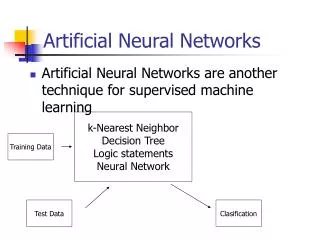
Explore the basic theory and structure of neurons in artificial neural networks, their functions, connections, and mathematical models. Learn how neurons work, classify data, and train a single-layer perceptron.

E N D
Artificial Neural Networks Basic Theory and Research Activity in KKU Dr. Nawapak Eua-anant Department of Computer Engineering Khon Kaen University 1 April 2546
Path I Basic Theory of Artificial Neural Network
A neuron : The smallest unit in the brain Cell body (soma) Dendrite Nucleus Neuron Axon Synapse Myelin sheath wThe brain consists of about 10,000 million neurons. Axon Hillock
A Neuron: The smallest unit in the brain (continued) Pictures from http://vv.carleton.ca/ ~neil/neural/neuron-a.html
A Neuron: The smallest unit in the brain (continued) Dendrite: w Each neuron contains approximately 10,000 dendrites connected to other neurons. wDrendrites receive “electrical signals” in from other neurons. w Some neurons have 200,000 connections or more. Axon: w Each axon consists of several terminal buttons called synapses connected to dendrites of other neurons. w The length of some axons may reach 1 meters. w Myelin sheets act as “insulator”.
Example of neurons w The cultured retinal explants taken from chick embryos From http://www.ams.sunysb.edu/research/pinezich/neuron_reconstruction/
Example of neurons (continued) w Neurons located in the cerebral cortex of the hamster. From http://faculty.washington.edu/chudler/cellpyr.html (Image courtesy of Dr. James Crandall, Eunice Kennedy Shriver Center)
How a neuron work 70 mV - + Organic ion Cl- K+ Na+ K+ Cl- Na+ w At the equilibrium point, there is a higher concentration of Potassium inside the cell and a higher concentration of sodium outside the cell. w This results in a potential across the cell membrane of about 70-100 mV called the resting potential.
How a neuron work (continued) -30 mV 70 mV - - + + Organic ion Organic ion Cl- Cl- K+ K+ Na+ Na+ K+ Cl- K+ Cl- Na+ Na+ + Before the depolarization w When the aggregate input is greater than the axon hillock's threshold value, there will be a large influx of sodium ion into the cell contributing to the depolarization. w This results in the action potential transmitted down the axon to other cells. Excitatory inputs + + + After the neuron has fired
Artificial Neural Network Input pattern Input nodes Output nodes Output pattern Hidden nodes Connections wIn ANN, each node is similar to a single neuron. w There are many connections Between nodes.
Mathematical Model of a Neuron x1 wi1 wi2 x2 yi S wi3 mi x3 McCulloch-Pitts model (1943) x = input Where g is the unit step function: m = the threshold level. w = weight of the connection
How can we use a mathematical function to classify ? Height (cm.) 180 140 40 Weight (kg.) 80 w Consider a simple problem: How can we classify fat and thin peoples? Thin Decision line Fat
How can we use a mathematical function to classify ? (cont.) w We used 2 inputs, weight (x1) and height (x2), to classify “thin” and “fat”. Thin Decision line x2 (cm.) Fat 180 Area where x2 - x1 - 100 > 0 w We can use a line to classify Data. Line x2 - x1 - 100=0 Area where x2 - x1 - 100 < 0 140 40 x1 (kg.) 80 Weight-height space
How can we use a mathematical function to classify ? (cont.) w The decision function to classify “thin” and “fat”: which is similar to the McCulloch-Pitts model: where Advantage: Universal linear classifier Problem: For a particular problem, how can we choose suitable weights w and m of the function ?
A Single Layer Perceptron: Adaptive linear classifier Adjust weights x1 wi1 x2 y - wi2 wi3 + x3 Desired output Rosenblett (1958) purposed a model with supervised learning: Error Network output S Input
A Single Layer Perceptron (continued) x1 wi1 wi2 x2 yi wi3 x3 wi4 x4 For each node, the output is given by Input layer Output layer wij= Connection weight of branch (i,j) xj = Input data from node j in the input layer mi = Threshold value of node i in the output layer g = Activation function
A Single Layer Perceptron (continued) 1.2 1 0.8 0.6 0.4 0.2 0 -0.2 -10 -5 0 5 10 1.2 1 0.8 0.6 a = 4 0.4 0.2 a = 2 a = 1 0 -0.2 a = 0.5 -10 -5 0 5 10 • w The number of input nodes depends on the number • of components of an input pattern. • w There are many types of activation functions. • For example: • The threshold function • The sigmoid function
How a Single Layer Perceptron Works w1 x1 y x2 w2 x2 x1 Consider a 2-input single layer perceptron with the threshold activation function. The output y is given by Decision Line L: Region where y = 1 w Slope and position of Line L depend on w1, w2 and m. Region where y = 0
How a Single Layer Perceptron Works (continued) x2 y =1 x1 y = 0 w The decision line must be suitably set for each problem. In other words, weights of the network must be selected properly. Example: Function AND The lines in this range can be used as Function AND. (1,1) (0,1) This line cannot be used for Function AND. (0,0) (1,0)
1. Feed input data into the network 2. Compute network output 3. Compute error 4. Adjust weights 5. Repeat step 1 until Training the Perceptron w Weights of the network must be adjusted in the direction To minimize error: Procedure for training the network
Training the Perceptron (continued) Updating weights using the Gradient descent method For a single layer perceptron with the thresholding Activation function,
1.2 1 0.8 0.6 x2 0.4 0.2 0 -0.2 -0.2 0 0.2 0.4 0.6 0.8 1 1.2 x1 Training the Perceptron (continued) Example: Function AND Iteration 16 OK! Iteration 12 Iteration 8 Iteration 4 Start Initial weights w1 = 0.5 w2 = 2.5 m = 1.0 a = 0.2
x2 Class y =1 (1,1) (0,1) (0,0) (1,0) x1 Class y = 0 Linearly separable data w In 2-dimensional space, a decision function of a single layer perceptron is a line. w Therefore, data to be classified must be separated using a single line. w We say that data is linearly separable.
x2 (1,1) (0,1) Class y = 1 Class y =0 x1 (0,0) (1,0) Nonlinearly separable data : Limitation of a single layer perceptron w There are some cases that a single layer perceptron does not work. w In such cases, we cannot use a single line to divide data between classes. The data is nonlinearly separable. Example: Function XOR Not OK!
Linearly separable vs. Nonlinearly separable Linearly separable Nonlinearly separable
x3 Class A Class B x2 x1 Higher Dimensional Space In the case of input patterns having more than 1 components, the output of the network is given by The decision function becomes the hyperplane: Example: 3D case Decision plane
Updating equation for the Gradient Descent Method Learning rate Input Output error Derivative Derivatives for some activation functions: 1. Linear unit 2. Sigmoid function 3. Tanh() function
A Multilayer Layer Perceptron Feed forward network Output nodes Layer N Layer N-1 Hidden nodes Layer 1 Connections Input nodes Layer 0 N-layer network
A Multilayer Layer Perceptron (continued) Back propagation algorithm Error Network output S - Input + Feed forward network Desired output
How A Multilayer Layer Perceptron works: XOR Example y1 x1 o x2 y2 Function XOR Layer 1 Layer 2 g( ) = threshold function
How A Multilayer Layer Perceptron Work (cont.) y1 x1 (1,1) (0,1) x2 y2 x2 (0,0) (1,0) x1 At the first layer Outputs at layer 1 w 2 nodes in the first layer correspond to 2 lines
How A Multilayer Layer Perceptron Work (cont.) y1-y2 space x1-x2 space (1,1) (0,1) y2 x2 (0,0) (1,0) x1 y1 Class 0 Class 1 At the first layer (1,1) Linearly separable ! (0,0) (1,0) w Hidden layers transform input data into linearly separable data !
How A Multilayer Layer Perceptron Work (cont.) y1 (1,1) o y2 y1-y2 space y2 (0,0) (1,0) y1 Class 0 Class 1 At the output layer w Space y1-y2 is linearly separable. Therefore the output layer can classify data correctly.
Back Propagation Algorithm The Gradient Descent Method Where Updating weights and bias
Example : Application of MLP for classification MATLAB Example Input points (x1,x2) generated from random numbers x = randn([2 200]); o = (x(1,:).^2+x(2,:).^2)<1; Desired output if (x1,x2) lies in a circle of radius 1 centered at the origin then o = 1 else o = 0 x2 x1
Example : Application of MLP for classification (cont.) Network structure Output node (Sigmoid) x1 Input nodes x2 Threshold unit (for binary output) Hidden nodes (sigmoid)
Example : Application of MLP for classification (cont.) Matlab command : Create a 2-layer network PR = [min(x(1,:)) max(x(1,:)); min(x(2,:)) max(x(2,:))]; S1 = 10; S2 = 1; TF1 = 'logsig'; TF2 = 'logsig'; BTF = 'traingd'; BLF = 'learngd'; PF = 'mse'; net = newff(PR,[S1 S2],{TF1 TF2},BTF,BLF,PF); Range of inputs No. of nodes in Layers 1 and 2 Activation functions of Layers 1 and 2 Training function Learning function Cost function Command for creating the network
Example : Application of MLP for classification (cont.) Matlab command : Train the network No. of training rounds net.trainParam.epochs = 2000; net.trainParam.goal = 0.002; net = train(net,x,o); y = sim(net,x); netout = y>0.5; Maximum desired error Training command Compute network outputs (continuous) Convert to binary outputs
Example : Application of MLP for classification (cont.) Initial weights of the hidden layer nodes (10 nodes) displayed as Lines w1x1+w2x2+q = 0
Example : Application of MLP for classification (cont.) Training algorithm: Levenberg-Marquardt back propagation Graph of MSE vs training epochs (success with in only 10 epochs!)
Example : Application of MLP for classification (cont.) Results obtained using the Levenberg-Marquardt Back propagation algorithm Unused node Only 6 hidden nodes are adequate ! Classification Error : 0/200
Pattern Recognition Applications Path II ANN Research in Department of Com. Eng. Khon Kaen University 1. Face Recognition Project 2. Resonant Inspection Project 3. Other Projects
Elements of Pattern Recognition Used to reduce amount of data to be processed by extracting important features of raw data. This process can reduce computational cost dramatically. Data acquisition Feature extraction Recognition process ANN
Face Recognition Project Senior Project 2001 1. Chavis Srichan, 2. Piyapong Sripikul 3. Suranuch Sapsoe 1. Possessing multi-resolution analysis capability that can eliminate unwanted variations of the facial image in wavelet scale-space. 2. Being able to compress the image using few coefficients Feature Extraction Discrete Wavelet + Fourier Transform Neural Network
Multiresolution Analysis Using Wavelet HL2 HL1 LH2 HH2 LH1 HH1 LL2 Original image L = Low frequency Component H = High frequency component 2-level multiresolition decomposed image
Feature Extraction OF Facial Images Original image 640x480 pixels 1. Segmentation Eliminates unwanted pixels 2. DWT 4 levels Reduces size of the image to 40x30 pixels 3. FFT Transforms to Freq. domain
Recognition Process FFT image Network output 2-layer feed forward network (120-10-1) Database of Facial images
Identification Results 90 % Match 24 % Match