Simplex Method and Sensitivity Analysis in Linear Programming by Doua Nassar
Understanding linear programming models and the simplex method. Learn how to convert inequalities into equations and tackle unrestricted variables. Transition from graphical to algebraic solutions.

Simplex Method and Sensitivity Analysis in Linear Programming by Doua Nassar
E N D
Presentation Transcript
Chapter 3 The Simplex Method and Sensitivity Analysis Doua Nassar
Simplex Method • Also called simplex technique or simplex algorithm • It is universal that is any linear model for which the solution exists can be solved by simplex method • The simplex method attempts to move from one corner point of the solution space to a better corner point until the optimum is found Doua Nassar
3.1 LP model in equation form (standard form) • All variables are non-negative • The right-hand side of each constraint is non-negative • All constraints are expressed as equations (=) • Objective function may be of maximization or minimization type • Unrestricted variables or unconstrained variables Doua Nassar
3.1.1 Converting Inequalities into Equations with Non-negative Right-hand side Two types of variables: i) Slack or unused variable (inequality <) ii) Surplus or extra variable (inequality >) Doua Nassar
i) Slack or unused variable (inequality <): - The difference between the Right-Hand Side (R.H.S) and Left-Hand Side (L.H.S) of the (inequality <) constraint thus yields the unused or slack amount of the resource. R.H.S - L.H.S = slack or unused amount - To convert the (inequality <) to an equation (=), a non-negative slack variable is added to the left-hand side of the constraint. Example of Reddy Mikks model: Constraint of raw material M1, (L.H.S) 6x1 + 4x2< 24 (R.H.S) Let s1 be the slack or unused amount of raw material M1, (L.H.S) 6x1 + 4x2 + s1 = 24 (R.H.S) s1 > 0 (non-negative slack variable) or 24 - (6x1 + 4x2 ) = s1 Doua Nassar
ii) Surplus or extra variable (inequality >): - The difference between the Left-Hand Side (L.H.S) and Right-Hand Side(R.H.S) of the (inequality >) constraint thus yields the surplus or extra amount of the resource. L.H.S - R.H.S = surplus or extra amount - To convert the (inequality >) to an equation (=),a non-negative surplus variable is subtracted from the left-hand side of the constraint. Example: (L.H.S) 5x1 + 7x2> 30 (R.H.S) Let s2 be the surplus or extra amount , (L.H.S) 5x1 + 7x2-s2 = 30 (R.H.S) s2 >0(non-negative surplus variable) or5x1 + 7x2 - 30=s2 Doua Nassar
Right-hand side of the constraint to be non-negative: Example: First method:- (L.H.S) - 3x1 + 2x2>-15 (R.H.S) Convert to equation (=), (L.H.S) - 3x1 + 2x2-s1 = -15 (R.H.S) s1 > 0 Multiply both sides of the equation by -1 to get non-negative right-hand side , 3x1 - 2x2 + s1 = 15 Second method:- (L.H.S) - 3x1 + 2x2>-15 (R.H.S) Multiply both sides of the constraint by -1 to get non-negative right-hand side , (L.H.S) 3x1 - 2x2< 15 (R.H.S) Convert to equation (=), 3x1 - 2x2 + s1 = 15 s1 > 0 Both equation and equation are same. 1 2 1 2 Doua Nassar
3.1.2 Dealing with unrestricted or unconstrained variables - Unrestricted or unconstrained variables can be either positive , negative or zero. • If a variable is unrestricted or unconstrained, it is expressed as the difference between two non-negative variables. - If x2 is unrestricted variable then it can be expressed as the difference between y1 non-negative variable and y2 non-negative variable, x2 = y1 – y2 where y1 >0 and y2 >0 Value of x2 unrestricted variable is either positive , zero or negative depending upon whether y1 is larger , equal to or smaller than y2 . Doua Nassar
Example: Express the following LP problem in the standard form: Maximize z = 4x1+ 6x2 + 2x3 subject to 2x1+ 5x2 < 6 x1+ 9x2- 7x3 < 8 4x1- 10x2 + 2x3 > 3 x1> 0 , x2> 0 Solution: Here x1 and x2 are restricted to be non-negative variables while x3 is unrestricted variable. Let x3 = y1 – y2 where y1 >0 and y2 >0 , then above LP problem can be written as, Maximize z = 4x1+ 6x2 + 2(y1 – y2) subject to 2x1+ 5x2 < 6 x1+ 9x2- 7(y1 – y2)< 8 4x1- 10x2 + 2(y1 – y2)> 3 x1> 0 , x2> 0, y1 >0, y2 >0 Doua Nassar
or Maximize z = 4x1 + 6x2 + 2y1 – 2y2 subject to 2x1 + 5x2 < 6 x1 + 9x2- 7y1 + 7 y2< 8 4x1 - 10x2 + 2y1 –2 y2> 3 x1> 0 , x2> 0, y1 >0, y2 >0 Including slack and surplus variables, the standard form is , Maximize z = 4x1 + 6x2 + 2y1 – 2y2 subject to 2x1 + 5x2 + s1 = 6 x1 + 9x2- 7y1 + 7 y2+s2 = 8 4x1 - 10x2 + 2y1 –2 y2- s3 = 3 x1> 0 , x2> 0, y1 >0, y2 >0 , s1>0 , s2>0 , s3>0 Doua Nassar
3.2 Transition from Graphical to Algebraic Solution - LP Solution by Graphical method is obtained by the corner points of the feasible space satisfying all the constraints. - For transition from graphical to algebraic method , the solution space is represented by m simultaneous linear equations and n non- negative variables. Doua Nassar
In algebraic representation: • The number of equations m is always less than or equal to the number of variables n . • If m=n , and the equations are consistent, the system has only one solution. e.g. The equation x = 2 has m=n=1 , the solution is unique. • If m < n (which represents the majority of LPs), then the system of equations , again if consistent, will yield an infinite number of solutions . e.g. The equation x + y =1 has m=1 and n=2, it yields an infinite number of solutions (any point on the line x + y = 1 is a solution). • If the number of equations m is larger than the number of variables n, then at least m – n equations must be redundant. Doua Nassar
Below gives a parallel steps for the algebraic and graphical method of solutions: Doua Nassar
Algebraic Determination of Corner Points - The LP solution space is represented algebraically by finding the candidates (corner points) for the optimum. - The corner points are determined by the simultaneous linear equations as follows: In a set of mxn (m < n) where m = number of equations and n =number of non-negative variables) , * set (n – m)variables equal to zero * solve the m equations for the remaining from n variables * if solution is unique, or there may be more solutions , it is called basic solution , but they must correspond to the corner points (feasible or infeasible) of the solution space. * the maximum number of Corner Points or basic solutions (feasible or infeasible) can be determined by the formula, Doua Nassar
To understand the above points, let us solve. Example 3.2-1 Consider the following LP with two variables: Maximize z = 2x1 + 3x2 subject to 2x1 + x2< 4 X1 + 2x2< 5 X1 , x2> 0 Note: Example 3.2-1 is explained by the file names Example 3.2-1 part 1 , Example 3.2-1 part 2 and Example 3.2-1 part 3 . Doua Nassar
Some important definitions:- Solution: A set of variables xj (j = 1,2,3,4,……n) is called a solution to the LP problem if it satisfies the constraints. Feasible Solution: A set of variables xj (j = 1,2,3,4,……n) is called a feasible solution to the LP problem if it satisfies the constraints as well as non-negativity restrictions xj > 0 (j = 1,2,3,4,……n) , si > 0 (i = 1,2,3,4,……m) . Non-Basic Variables: Set (n – m)variables equal to zero are called non-basic variables. Basic Variables: The values of remaining from n variables (some of them may be zero) are called basic variables. Doua Nassar
Basic Solution: A solution obtained by setting (n – m)variables equal to zero and solving of remaining from n variables (some of them may be zero) is called a basic solution . (Together non-basic variables and basic variables give a basic solution). Basic Feasible Solution: A basic solution which is feasible, is said to be a basic feasible solution. Non-Degenerate Basic Feasible Solution: It is a basic feasible solution in which all the basic variables are positive or non-zero ( value of basic variable > 0) . Degenerate Basic Feasible Solution: It is a basic feasible solution in which one or more of the basic variables are equal to zero ( value of basic variable = 0) . Doua Nassar
Optimal Solution: A basic feasible solution is said to be optimal if it optimizes the objective function. Convex Set in Linear Programming (LP): The feasible solution space is said to form a convex set, if for any two feasible points in the set ,the line segment joining any two feasible points lies entirely in the set. Extreme Point (Corner Point): Every basic feasible solution of a LP is an extreme point of the convex set of feasible solutions and every extreme point is a basic feasible solution of the set of the constraints. Doua Nassar
Convex set Non-convex set Doua Nassar
3.3 The Simplex Method Algebraically method finds all the basic solutions or corner points of the LP problem. The Simplex method only finds few of the basic solutions or corner points of the LP problem. Doua Nassar
3.3.1 Iterative Nature of the Simplex Method For maximize z: Normally , the simplex method starts at the origin (0,0) where x1 = 0 , x2 = 0 . Both x1 and x2 are non-basic variables. At this starting point the value of the objective function z = 0 . In an objective function z it is to be decided which of the two non-basic variables above their current zero values can improve (increase) the value of z. In simplex method one non-basic variable is increased at a time. The non-basic variable which has the largest rate of improvement in z is selected. Doua Nassar
For minimize z: • Both x1 and x2 are non-basic variables. • In an objective function z it is to be decided which of the two non-basic variables can improve (decrease) the value of z. • In simplex method one non-basic variable is decreased at a time. • The non-basic variable which has the smallest rate of improvement in z is selected. - Either x1 or x2 will be selected in the objective function z which has the smallest rate of improvement . Doua Nassar
Example 3.2-1: Maximize z = 2x1 + 3x2 - The objective function z shows that an increase in either x1 or x2 or both above their current zero values will improve(increase) the value of z. • The rate of improvement in z is 2 for x1 and 3 for x2 . • We therefore select to increase x2 , the variable with the largest rate of improvement. Doua Nassar
Figure 3.4 Iterative process of the simplex method of Example 3.2-1 Doua Nassar
The figure 3.4 shows that the value of x2 will be increased from point A origin until corner point B is reached. • At point B simplex method will then increase the value of x1 to reach the improved corner point C, which is the optimum. • The path of the simplex method is thus defined as A B C . - Each corner point along the path is associated with an iteration. • Simplex method moves alongside the edges of the solution space which means that the method cannot cut across the solution space, for example going from A to C directly cannot be done. Doua Nassar
We need to make transition from graphical solution to the algebraic solution by showing how the points A , B and C are represented by their basic and non-basic variables . • The following table summarizes these representations: Corner point Basic variables Non-basic (zero) variables A s1 , s2 x1, x2 B s1 , x2 x1, s2 C x1, x2 s1 , s2 Doua Nassar
We can notice that there is a change pattern in the basic and non-basic variables as the solution moves along the path A B C . • In simplex method there are entering and leaving variables. • Entering variable means that variable which is going from non-basic variable to basic variable. • Leaving variable means that variable which is going from basic variable to non-basic variable. Doua Nassar
From A to B x2 is the entering variable because it enters the basic solution . • From A to B s2 is the leaving variable because it leaves the basic solution . • From B to C x1 is the entering variable because it enters the basic solution . • From B to C s1 is the leaving variable because it leaves the basic solution . Corner point Basic variables Non-basic (zero) variables A s1 , s2 x1, x2 B s1 , x2 x1, s2 C x1, x2 s1 , s2 Note: Path of three examples has been explained by the file name Three examples of path . Doua Nassar
3.3.2 Computational Details of the Simplex Algorithm - The computational details of a simplex iteration explains rules for determining the entering and leaving variables as well as for stopping the computations when the optimum solution has been reached. Example 3.3-1 Note: Example 3.3-1 has been explained by the file names Example 3.3-1 part 1 , Example 3.3-1 part 2 , Example 3.3-1 part 3 , Example 3.3-1 part 4 and Example 3.3-1 part 5 . Doua Nassar
Example 3.3-2 Find all the basic solutions to the following problem. Also find which of the basic solutions are (i) basic feasible solution (ii) non-degenerate basic feasible solution (iii) optimal basic feasible solution. Maximize z = x1 + 3x2 + 3x3 subject to x1 + 2x2 + 3x3 = 4 2x1 + 3x2 + 5x3 = 7 x1 , x2 , x3 > 0 1 2 Doua Nassar
Solution: - Here m = 2 ( number of equations) , n = 3 (number of non-negative variables) . - Total number of corner points or basic solutions are, C = 3!___ = 3!___ = 3 X 2 X 1_ = 3 2!(3-2)! 2! 1! 2 X 1 X 1 - Number of non-basic variables are, n – m = 3 – 2 = 1 - When x1 = 0 (non-basic variable), then x2 and x3 are basic variables. Put x1 = 0 in equations and to get values of x2 and x3 , x1 + 2x2 + 3x3 = 4 2x1 + 3x2 + 5x3 = 7 1 2 1 2 Doua Nassar
1’ 2’ Now equations become, 2x2 + 3x3 = 4 3x2 + 5x3 = 7 Multiply eq by 3 and eq by 2 , 6x2 + 9x3 = 12 6x2 + 10x3 = 14 Subtract eq from eq , 6x2 + 10x3 = 14 + 6x2+ 9x3 = +12 ___________________ x3 = 2 1’ 2’ 1’’ 2’’ 1’’ 2’’ 2’’ 1’’ Doua Nassar
1’ 1’ Put x3 = 2 in eq to get value of x2, 2x2 + 3x3 = 4 2x2 + 3(2) = 4 2x2 + 6 = 4 2x2 = 4 – 6 x2 = -2 2 x2 = -1 Therefore x1 = 0 , x2 = -1 and x3 =2 Doua Nassar
1 2 - When x2 = 0 (non-basic variable), then x1 and x3 are basic variables. Put x2 = 0 in equations and to get values of x1 and x3 , x1 + 2x2 + 3x3 = 4 2x1 + 3x2 + 5x3 = 7 Now equations become, x1 + 3x3 = 4 2x1 + 5x3 = 7 1 2 1’ 2’ Doua Nassar
1’ 1’’ 2’ 1’’ 1’’ Multiply eq by 2 , 2x1 + 6x3 = 8 Subtract eq from eq , 2x1 + 6x3 = 8 + 2x1+ 5x3 = + 7 ___________________ x3 = 1 Put x3 = 1 in eq to get value of x1, x1 + 3x3 = 4 x1 + 3(1)= 4 x1 + 3= 4 x1 = 4 – 3 x1 = 1 Therefore x1 = 1 , x2 = 0 and x3 = 1 2’ 1’ 1’ Doua Nassar
1 2 - When x3 = 0 (non-basic variable), then x1 and x2 are basic variables. Put x3 = 0 in equations and to get values of x1 and x2 , x1 + 2x2 + 3x3 = 4 2x1 + 3x2 + 5x3 = 7 Now equations become, x1 + 2x2= 4 2x1 + 3x2= 7 Multiply eq by 2 , 2x1 + 4x2= 8 1 2 1’ 2’ 1’ 1’’ Doua Nassar
2’ 1’’ 1’’ 2’ Subtract eq from eq , 2x1 + 4x2 = 8 + 2x1+ 3x2 = + 7 __________________ x2 = 1 Put x2 = 1 in eq to get value of x1, x1 + 2x2= 4 x1 + 2(1) = 4 x1 + 2 = 4 x1 = 4 – 2 x1 = 2 Therefore x1 = 2 , x2 = 1 and x3 = 0 1’ 1’ Doua Nassar
Serial Non-basic Basic Basic Basic Non-degenerate Objective number variables variables solution feasible basic feasible value solution solution z_____ 1 x1 (x2,x3) (-1,2) No No - 2 x2 (x1,x3) (1 ,1) Yes Yes 4 3 x3 (x1,x2) (2, 1) Yes Yes 5 Optimal basic feasible solution is number 3 which gives maximize z = 5 where x1 = 2 ,x2 = 1 and x3= 0 . Doua Nassar
Example: Find the solution of the LP problem algebraically. Max Z=2x1+3x2 ST. 2x1 + x2 <4 x1 + 2x2 <5 x1 , x2>0 Doua Nassar
Example: Solve the following LP problem by simplex method. Max z = 5x1- 4x2 subject to 6x1 + 4x2 <24 x1- 2x2 <6 -x1+ x2 <1 x2 <2 x1 , x2 >0 Doua Nassar
Solution: 1- Convert constraints to equation or standard form. Max z = 5x1- 4x2 subject to 6x1 + 4x2 + s1 = 24 x1 - 2x2 + s2 = 6 -x1 + x2 + s3 = 1 x2 + s4 = 2 x1 , x2 , s1 , s2 , s3 , s4>0 Doua Nassar
2- Put the coefficient of equation in a table Doua Nassar
3- Determine Entering variable. Entering variable - max negative number in the objective Entering variable Doua Nassar
4- Find the Leaving variableCalculate Sol col. / Pivot col. (entering variable)Take the smallest positive value Entering variable Leaving variable Doua Nassar
5- Find the Pivot value , Pivot ElementPivot Value= Entering Variable Col Leaving Variable RowPivot Element = Leaving variable Row / Pivot valuePivot Value = 6Pivot Element = (6, 4, 1, 0, 0, 0, 24) / 6 =( 1, 4/6, 1/6, 0, 0, 0, 4) Doua Nassar
6- Gauss-Jordan row operations: 1.Replace the leaving variable in the Basic column with the entering variable. 2. All other rows , including z: New row = Current row – {(Pivot column co-efficient) X (New pivot row)} - s2 -row: (1, 2, 0, 1, 0, 0, 6) – (1)(1 , 4/6, 1/6, 0,0,0,4) = (0, 4/3, -1/6, 1, 0, 0, 2) Make it for all rows THE RESULT….. Doua Nassar
Now take a look to Z row if you get a positive and zero values stop work IF not Repeat all steps from step 3 until you reach positive or zeros values Doua Nassar
Entering variable Leaving variable Doua Nassar