Download
1 / 17
170 likes | 444 Vues
Berry & Associates // Spatial Information Systems 2000 S. College Ave, Suite 300, Fort Collins, CO 80525 Phone: (970) 215-0825 Email: jberry@innovativegis.com …visit our Website at www.innovativegis.com/basis.

E N D
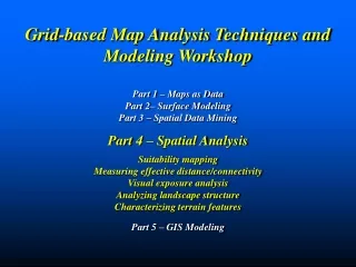
Berry & Associates // Spatial Information Systems2000 S. College Ave, Suite 300, Fort Collins, CO 80525Phone: (970) 215-0825 Email: jberry@innovativegis.com…visit our Website atwww.innovativegis.com/basis Grid-based Map Analysis and GIS ModelingUnderstanding Spatial Patterns and Relationships Intermediate Workshop Presented byJoseph K. Berry “Map Analysis and GIS Modeling is technical Oz …you’re hit with a tornado of new concepts, then come back to yourself a short time later wondering what on earth all those crazy things meant” Part 1 – Introduction and Data Considerations Part 2 – Spatial Analysis Techniques and Considerations Part 3 – Spatial Statistics Techniques and Considerations Part 4 – GIS Modeling Approaches and Considerations
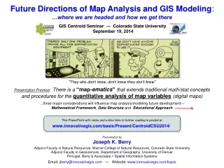
Geographic Information Systems Global Positioning System Remote Sensing Today’s Focus Mapping involves precise placement (delineation) of physical features (graphical) Analysis involves investigation of spatial relationships (numerical) Descriptive Mapping Prescriptive Modeling (Nanotechnology) Geotechnology (Biotechnology) Geotechnology is one of the three "mega technologies" for the 21st century and promises to forever change how we conceptualize, utilize and visualize spatial information in research, education and commercial applications GPS/GIS/RS WhereisWhat WhyandSo What (Berry)
Manual Mapping for 8,000 years Computer Mappingautomates the cartographic process (70s) (digital slide show WorldZoom) Spatial Database Managementlinks computer mapping techniques with traditional database capabilities (80s) (digital slide show RealEstate) Map Analysisrepresentation of relationships within and among mapped data (90s) …the focus of today’s workshop Historical Setting and GIS Evolution GIS = Geographic Information Systems …a more recent expression of mapping (40 years) Multimedia Mappingfull integration of GIS, Internet and visualization technologies (00s) …but that’s another story (Berry)
Click on… Info Tool Theme Table Distance Zoom Pan Select Theme Spatial Table Geo-Query… Query Builder : Object ID X,Y X,Y X,Y : …identify tall aspen stands Attribute Table FeatureSpeciesetc. : : Object ID Aw : : Big …over 400,000m2 (40ha)? Discrete, irregular map features (objects) Desktop Mapping Framework (Vector, Discrete) (Berry)
Spatial Table (spatial objects) Where Hole 2)Special Punch was used to notch-out the hole assigned to a particular characteristic (attribute), such as #11 notch = Douglas fir timber type Notch #11 15 14 13 12 10 9 8 7 Hole 6 Cards pulled up… … DO NOT have characteristic 5 4 3 2 Index card (tray) 1 Query Tray holds all of the index cards for a project area #57 Notch Cards falling down… … HAVE characteristic #57 Timber Stand Map (wall) 5)Card ID# identifies the timber stand polygons from the search and the appropriate locations are shaded— …a “Database-entry Geo-query” Manual GIS (Geo-query circa 1950) 1)Index Card with series of numbered holes around the edge and written description/data in the center 3)Pass a long Needle through the stack of cards and lift… Data Table (attribute records) What 4)Repeat using the search results sub-set for more characteristics (Berry)
Click on… Shading Manager Zoom Pan Rotate Display Grid Analytics… Map Analysis …calculate a slope map and drape on the elevation surface Grid Table : --, --, --, --, --, --, --, --, --, --, --, --, --, 2438, --, --, --, --, --, : Continuous, regular grid cells (objects) Points, Lines, Polygons and Surfaces MAP Analysis Framework(Raster, Continuous) (Short Exercise #1) (Berry)
Calculating Slope and Flow (Map Analysis) Inclination of a fitted plane to a location and its eight surrounding elevation values Slope (47,64) = 33.23% Slope map draped on Elevation Slope map % Flow (28,46) = 451 Paths Elevation Surface Total number of the steepest downhill paths flowing into each location Flow map draped on Elevation (Berry) Flow map (Berry)
Erosion Potential Reclassify Overlay Reclassify Erosion_potential Slopemap Slope_classes Flow/Slope Reclassify Simple Buffer Flowmap Flow_classes Protective Buffers …reach farther in areas of high erosion potential But all buffer-feet are not the same… (slope/flow Erosion_potential) Streams Simple Buffer Erosion_potential Deriving Erosion Potential & Buffers (Berry)
Distance away from the streams is a function of the erosion potential (Flow/Slope Class) with intervening heavy flow and steep slopes computed as effectively closer than simple distance— “as the crow walks” Distance Effective Erosion Distance Erosion Buffers Close Far Simple Buffer Heavy/Steep (far from stream) Erosion_potential Light/Gentle (close) Effective Buffers (digital slide show VBuff2) Streams Calculating Effective Distance(variable-width buffers) (Berry)
Simple erosion potential model– based on terrain slope and flow (Short Exercise #2) Workshop CD Bighorn_erosion.scr Script See Default.htm …extended to derive a Variable-width Buffer (Full Exercise #2) Erosion Potential Buffer Model(MapCalc script) (Berry)
…a Grid Map consists of a matrix of numbers with a value indicating the characteristic or condition at each grid cell location—geo-registered set of Grid Layers Lines Layer Mesh Grid Map Fill …the Analysis Frame provides consistent “parceling” needed for map analysis and extends Points, Lines and Areas to Surfaces Basic Grid Structure (Berry)
Display Types Display Form— 2D or 3D Display Structure — Grid or Lattice Display Data Type — Discrete or Continuous Recognizing Data & Display Types • Data Types • Numerical Distribution— • Nominal, Ordinal (Qualitative) • Interval, Ratio (Quantitative) • Binary (Boolean) • Geographical Distribution— • Choropleth (Discrete) • Isopleth (Continuous) (Berry)
V to R– burning the points, lines and areas into the grid (fat, thin and split) Points— Containing Cell Lines Polygons Points— Cell Centroid R to V– connecting grid centroids, sides and edges (line smoothing) Vector to/from Raster Old saying—“…raster is faster, but vector is corrector” Vector— “precise” placement of spatial objects Grid— “accurate” characterization of spatial relationships (Berry)
Handheld GPS unit Accuracy describes the closeness of arrows to the bull’s-eye at the target center (actual/correct) High Accuracy but Low Precision Accuracyvs.Precision …the “target analogy” compares measurements to the pattern of arrows shot at a target High Precision but Low Accuracy Precision GPS unit Precision relates to the size of the cluster of arrows— grouped tightly together is considered precise Accuracy versus Precision The Wikipedia defines Accuracy as “the degree of veracity” (exactness) while Precision as “the degree of reproducibility” (repeatable) (Berry)
Interpreter A Interpreter B Interpreter C Vegetation Parcel Mapping Superimposed interpretation boundaries Accuracy = classification (What) Precision = delineation (Where) Photo Interpreter A Cottonwood Photo Interpreter C Cottonwood Photo Interpreter B Ponderosa Pine Classification versus Delineation (spatial perspective) Classification Accuracy (What) Delineation Precision (Where) (Berry)
Routing Criteria Most Preferred Least Preferred 1 2 3 4 5 6 7 8 9 Housing Density Road Proximity Sensitive Areas Visual Exposure RP & SA times 10 HD & RP times 10 HD & VE times 10 Environmentalists Engineers Homeowners Start Start Optimal Path Optimal Corridor Engineers Environmentalists Homeowners Average of the three cost surfaces Combined Solution Individual Solutions End End Model Accuracy/Precision (spatial modeling perspective) Calibrate Expert Opinion …cognitive mapping has no definitive right/wrong solution— Most Preferred Weight Stakeholder Values (Berry)
…but before we leave Introduction & Data Considerations to tackle Spatial Analysis (operations for reclassify, overlay, distance and neighbors), any… Questions? Questions? (Berry)