Optimizing Compiler Techniques: Static and Dynamic Profilers for Effective Code Generation
This document explores the intricacies of optimizing compilers, focusing on both static and dynamic profiling techniques. It emphasizes the importance of memory management, internal representation, and various code optimizations such as scalar and loop optimizations. The discussion includes the profitability of intraprocedural optimizations, highlighting examples like common subexpression elimination and control flow graph behavior. It also examines the significance of analyzing execution probabilities for various code segments to enhance optimization decisions.

Optimizing Compiler Techniques: Static and Dynamic Profilers for Effective Code Generation
E N D
Presentation Transcript
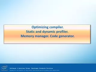
Optimizing compiler.Static and dynamic profiler. Memory manager. Code generator.
Source files FE (C++/C orFortran) Internal representation Profiler Temporary files or object files with IR Scalar optimizations Loop optimizations Interprocedural optimizations Code generation Scalar optimizations Object files Code generation Loop optimizations Executable file of library
Determining the optimization profitability Profitability of intraprocedural optimizations depends on the statement execution probability. It closely relates with control flow graph behavior. Example for common subexpressions elimination. z=x*y; if(hardly_ever) { t=x*y; } This optimization has the disadvantage, it enlarges routine stack because it creates temporary variable to store the result of repeated calculation. In the case when usage of this result is happened inside infrequent basic block the optimization can not be paid back. A similar argument is appropriate for loop invariant hoisting. for(i=0;i<n;i++) { … if(hardly_ever) { … = x*y; } }
A lot of optimizations need an information on probability of different events for more precise optimization profitability estimation: For intraprocedural optimization “field reordering” it is important to detect which fields are used together “frequently”. For inlining it is unprofitable to substitute a routine to a call site which is “rarely” used. For partial inlining compiler need to detect “hot” parts of the code inside the inline candidate routine. For vectorization it is unprofitable to vectorize loops with “small” iteration count. For efficient auto-parallelization compiler need to estimate amount of work which is performed on loop iteration. And so on … Thus optimizing compiler need methods for application event estimation. There are small hints which can be used to provide the additional information to compiler. For example, builtin_expect is designed to transfer the compiler information about the probability of branching if(x) => if(__builtin_expect(x,1))
Static profiler Static profiler performs a static program analysis. It is analysis of application source code performed without the application execution. Profiler calculates the probability of conditional jumps and the base blocks execution fequency. Routine execution frequency is calculated during the call graph analysis. Source code analysis can not provide an accurate calculation of the weight (execution frequency) characteristics. In general, the input of the executable program it is not known, the compilation time is limited. Nevertheless, the data obtained using the static profiler is used to perform various interprocedural optimizations.
Dynamic profiler Dynamic profiler calculates weights based on the analysis of statistics collected by an instrumented application during execution. To obtain benefits from dynamic profiler an application should be built with instrumentation. The instrumented application should be ran with a set of common data. The final build will use statistics collected during execution for more effective optimizations. /Qprof-gen[:keyword] instrument program for profiling. Optional keyword may be srcpos or globdata /Qprof-use[:<arg>] enable use of profiling information during optimization weighted - invokes profmerge with -weighted option to scale data based on run durations [no]merge - enable(default)/disable the invocation of the profmerge tool
Dynamic profiler and auto vectorization example #include <stdio.h> float ttt(float* vec,int n1, int n2) { int i; float sum=0; for(i=n1;i<n2;i++) sum+= vec[i]; return sum; } int main() { float zzz[1000]; int i; float sum=0; for(i=0;i<1000;i++) zzz[i]=i; for(i=1;i<1000;i=i+5) sum = sum+ttt(zzz,i,i+5); for(i=1;i<1000;i=i+6) sum = sum+ttt(zzz,i,i+6); printf("sum=%f\n",sum); } Let’s check if compiler is able to estimate vectorization profitability with dynamic profiler. icl -Ob0 test_vecpgo.c -Qipo -Qvec_report3 … test_vecpgo.c(6): (col. 2) remark: LOOP WAS VECTORIZED. icl -Ob0 test_vecpgo.c -Qipo -Qprof_gen test_vecpgo.exe icl -Ob0 test_vecpgo.c -Qipo -Qprof_use -Qvec_report3 … test_vecpgo.c(6): (col. 2) remark: loop was not vectorized: vectorization possible but seems inefficient.
Dynamic profiler and auto parallelization example Let’s check if compiler is able to estimate auto parallelization profitability with dynamic profiler. icl /Ob0 multip.cmain.c /O3 /Qipo /Qparallel /Qpar_report3 … procedure: matrix_mul_matrix multip.c(4): (col. 3) remark: loop was not parallelized: insufficient computational work. time multip.exe – 3.6s icl /Qprof_gen /Ob0 multip.cmain.c /O3 /Qipo /Qparallel multip.exe icl /Qprof_use /Ob0 multip.cmain.c /O3 /Qipo /Qparallel /Qpar_report3 procedure: matrix_mul_matrix multip.c(4): (col. 3) remark: LOOP WAS AUTO-PARALLELIZED. time multip.exe – 0.67s cat multip.c void matrix_mul_matrix(int n, double *C, float *A, float *B) { inti,j,k; for (i=0; i<n; i++) for (j=0; j<n; j++) for(k=0;k<n;k++) C[i*n+j]+=(double)A[i*n+k] * (double)B[k*n+j]; } cat main.c #include <stdio.h> #define N 2000 extern void matrix_mul_matrix(int,double *,float *,float *); int main() { float *A,*B; double *C; … matrix_mul_matrix(N,C,A,B); printf("%f\n",C[2*N+2]); }
Dynamic memory allocation and memory manager Objects and arrays can be allocated dynamically at runtime with the operators new() and delete(), functions malloc() and free(). The memory manager is part of the application, processing requests for the allocation and freeing of memory. A typical situations where dynamic memory allocation is necessary are: • Creation of a large array which size is unknown at compile time. • An array can be very large in order to place it on the stack. • Objects must be created at run time if the number of required objects is unknown. Disadvantages of dynamic memory allocation: • Allocating and freeing memory has its overhead. • Allocated memory becomes fragmented when objects of different types are allocated and released in unpredictable order. • If a size of allocated object should be changed but there is no possibility to extend the memory block, than the memory should be copied form old block to the new. • Garbage collection is necessary because memory blocks of required size can be not found because of memory fragmentation.
Important factor of the performance in C++ is a close memory placement of the objects belongs to same linked list. Linked list is less effective than the linear array for the following reasons: • Each object allocated separately. Allocation and release of the object has its price. • Objects memory placement is not sequential. The probability of cash hit is reduced when traversing lower than for array. • Need more memory to store references and information about the allocated memory block. According to the same reason continuous array is more profitable than array of pointers. A cash hit probablility can be different for different memory managers because of different method of memory allocation. For example, managers can combine allocated objects according to object size. There are some alternative memory managers such as SmartHeap or dlmalloc, which can provide better performance in some cases.
Linked list: • Linked lists in memory 4GB Can be allocated in memory: 2GB 0GB And in the physical memory: P1 P2 P3 P4
Memory manager for array of pointers for (i=0;i<N;i++){ a[i]->x = 1.0; b[i]->x = 2.0; a[i]->y = 2.0; b[i]->y = 3.0; a[i]->z = 0.0; b[i]->z = 4.0; } for(k=1;k<N;k++) for (i=k;i<N-20;i++){ a[i]->x = b[i+10]->y+1.0; a[i]->y = b[i+10]->x+a[i+1]->y; a[i]->z = (a[i-1]->y - a[i-1]->x)/b[i+10]->y; } printf("%d \n",a[100]->z); } #include <stdlib.h> #include <stdio.h> #define N 10000 typedefstruct { intx,y,z; } VecR; typedefVecR* VecP; int main() { inti,k; VecP a[N],b[N]; VecR *tmp,*tmp1; #ifndef PERF for(i=0;i<N;i++){ a[i]=(VecP)malloc(sizeof(VecR)); b[i]=(VecP)malloc(sizeof(VecR)); } #else tmp=(VecR*)malloc(sizeof(VecR)*N); tmp1=(VecR*)malloc(sizeof(VecR)*N); for(i=0;i<N;i++) { a[i]=(VecP)&tmp[i]; b[i]=(VecP)&tmp1[i]; } #endif iccstruct.c -fast -o a.out iccstruct.c -fast -DPERF -o b.out time ./a.out real 0m0.998s time ./b.out real 0m0.782s
There is a popular way in C++ to improve work with dynamically allocated memory through the use of containers. Creation and use of containers is one example of effective template use in C++. The most common set of containers provided by Standard Template Library (STL), which comes with a modern C++ compilers. It looks, however, the STL is mainly designed for flexibility of use and performance issues have a lower priority. Therefore, the expansion of container size is performed step by step and many containers doesn’t have a constructor allowing to define the initial memory amount should be allocated. In the case of expansion the container may need to copy the its contents. Such copy is performed via copy constructors and can make performance worse. A popular method for object memory allocation is memory pools method. In this case memcpy can be used for pool expansion.
Source files FE (C++/C orFortran) Internal representation Profiler Temporary files or object files with IR Scalar optimizations Loop optimizations Interprocedural optimizations Code generation Scalar optimizations Object files Code generation Loop optimizations Executable file of library
Code generator • Code generation (CG) is a part of the compilation process. Code generator converts correct internal representation into a sequence of instructions that can be run on the particular proccessor architecture. CG may apply different machine-dependent optimizations. Code generator can be a common part for a variety of compilers, each of which generates an intermediate representation as input to the code generator. • Basic actions: • Conversion of the internal representation to the instructions of given processor architecture. • Specific architectural optimization; • Simple intrinsic substitution (inline); • Basic blocks memory alignment; • Procedure calls preparations, load the appropriate variables to registers and/or to the stack for parameters passing; • The same for the called procedure. Local variable stack allocation. • Instruction scheduling; • Register allocation; • Jump distances calculation; • …
Register allocation One of the basic tasks of code generator is a register allocation. The register allocation is program variable mapping to the microprocessor register set. Register allocation can be performed inside a single basic block (the local register allocation), or the entire process (global register allocation). Typically, the number of variables in the program much greater than the number of available physical registers, so variables are stored in the memory and loaded to registers before usage. After usage register should be saved to memory. Memory exchange (register save/load operations) should be minimized for better performance; compiler should choose and hold in registers more frequently used variables. It is hard to determine frequency of use for different variables. A problem which causes loss of performance because of exchange between registers and memory is called register spilling. Register allocation is performed via interference graph coloring.
The implementation of register allocation with graph coloring contains the following steps: 1.) Identifying the live range of variables (A program region in which the variable is used) and gives each a unique name. 2.) Interference graph building. Each variable corresponds to a vertex. If the live ranges of variables intersect, then there is edge between these vertexes. Each vertex color should be different from the connected vertexes colors. Number of colors used relates to number of registers needed. 3.) Actual graph coloring. 4.) If the coloring fails then we need to break some vertex (this means storing register to memory during live range of variable) and retry graph coloring. The register allocation is better when the registers contains most frequently used data. Dynamic profiler information can be very useful for better register allocation.
Data dependence for register reuse Dependency issue was raised in previous lectures. Dependencies are used and calculated in order to prove the validity of the permutation optimizations. Code generator uses dependencies to identify opportunities for reusability of data in calculations. It allows to avoid unnecessary memory loads, and memory write backs. For example: DO I = 1, N A (I+1) = A (I) F (...) END DO It makes sense to tie A (I+1) with register, so the next iteration won't load A(I) from memory
Instruction scheduling It is a computer optimization which is used to improve the instructional parallelism level. This optimization is usually done by changing the order of instructions to reduce delays in the processor pipeline. Another reason for instruction scheduling can be an attempt to improve memory subsystem work by moving memory read far before it’s usage. Any processor contains its own mechanism for instruction planning and distribution across the execution units. This mechanism provides a proactive view of incoming instructions. But it can not be sufficiently effective because "window-ahead view" is limited. Instructions can be interchanged according to the following considerations: 1) Place memory read as far as possible before using the results; 2) Mixed instructions use different executable unit of the processor; 3) Closer instructions use the same variable to simplify the selection of registers. Planning regulations can be made within a single base unit, or within the superblock, combining several basic blocks. Some instructions can be moved beyond the boundaries of their base block. Instruction planning can be carried out before and after the allocation of registers.
An example of a processor and architectural optimization (using cmovne) Control flow dependence can be replaced by data dependence using cmovne. Branching disappears and it speeds up the badly predicted branches. #include <stdio.h> int main() { int volatile t1,t2,t3; inti,j,aa; int a[1000]; t1=t2=t3=0; aa=0; for(i=1;i<100000;i++) { for(j=1;j<1000;j++){ if(t1|t2|t3) aa=2; else aa=0; a[j]=a[j]+aa; t3=j%2; } } printf("%d\n",a[50]); } icctest.c -O2 -xP -o a.out time ./a.out 0m0.379s icctest.c -O2 -o b.out time ./b.out 0m0.441s -xP ( /QxP) use /QxSSE3 This example demonstrates how instruction set can change performance of application.
Assembler for better test: ..B1.3: # Preds ..B1.9 ..B1.2 movl 4008(%esp), %ebx #12.7 orl 4004(%esp), %ebx #12.10 movl $2, %edx #15.6 orl 4000(%esp), %ebx #12.13 movl $0, %ebx #15.6 cmovne %edx, %ebx #15.6 addl %ebx, (%esp,%eax,4) #16.14 movl %eax, %edx #17.9 andl $-2147483647, %edx #17.9 jge ..B1.9 # Prob 50% #17.9 # LOE eax edx ecx esi edi ..B1.10: # Preds ..B1.3 subl $1, %edx #17.9 orl $-2, %edx #17.9 addl $1, %edx #17.9 # LOE eax edx ecx esi edi ..B1.9: # Preds ..B1.3 ..B1.10 movl %edx, 4000(%esp) #17.4 addl $1, %eax #11.17 cmpl $1000, %eax #11.12 jl ..B1.3
Assembler for test without cmovne : ..B1.3: # Preds ..B1.9 ..B1.2 movl 4008(%esp), %ecx #12.7 orl 4004(%esp), %ecx #12.10 orl 4000(%esp), %ecx #12.13 movl $2, %ecx #15.6 jne ..L1 # Prob 50% #15.6 movl $0, %ecx #15.6 ..L1: # addl %ecx, (%esp,%edx,4) #16.14 movl %edx, %ecx #17.9 andl $-2147483647, %ecx #17.9 jge ..B1.9 # Prob 50% #17.9 # LOE eax edx ecx ebx esi edi ..B1.10: # Preds ..B1.3 subl $1, %ecx #17.9 orl $-2, %ecx #17.9 addl $1, %ecx #17.9 # LOE eax edx ecx ebx esi edi ..B1.9: # Preds ..B1.3 ..B1.10 movl %ecx, 4000(%esp) #17.4 addl $1, %edx #11.17 cmpl $1000, %edx #11.12 jl ..B1.3