Download
1 / 50
500 likes | 593 Vues
Explore how navigation in networks using local information relates to splicing in parasites. Discuss the importance of navigation in various network types, scale-free networks, navigation models, basins of attraction, and the distribution of basins in scale-free networks. Analyze the transition at γ=3 and the giant basin theory, as well as deterministic fractal (u,v)-nets and generalization to lattices. A fun exercise in probability and the Kleinberg model is also covered.

E N D
How are navigation in networks and splicing in parasites related? Shai CarmiBar-Ilan UniversityDepartment of physics and the faculty of life sciences Summer 2010, USA
Navigation in networks with local information • Navigation is important in communication networks, transportation networks, and social networks. • Knowledge of the entire network is usually not feasible. • Use greedy navigation. The Internet at the Autonomous Systems levelCarmi et. al, PNAS 104, 11150 (2007) MapQuest Boguna & Krioukov, PRL 102, 058701 (2009)
Scale-free networks • Nomenclature: In a network (graph), links (edges) connect nodes (vertices).The degree of a node, k, is its number of links. • In the last decade, measurements showed that almost all natural networks are scale-free. • Nodes in scale-free networks have degrees in all orders of magnitude, including nodes with an extremely large number of links (hubs). • Degree distribution: • Small γ: network is highly heterogeneous, many hubs exist. • Large γ: network is homogeneous, fewer hubs, similar to purely random networks.
Navigation models • Navigating to the hub.S. Carmi., P. L. Krapivsky, and D. ben-Avraham, Physical Review E 78, 066111 (2008). • Kleinberg’s navigation model.S. Carmi, S. Carter, J. Sun, and D. ben-Avraham. Physical Review Letters 102, 238702 (2009).
j How to find the most connected node in the network: an algorithm i l d a k • Start from a given node. • Go to the neighbor with highest degree(break ties arbitrarily). • Keep going, until reaching a peak- a node whose degree is greater than the degrees of all of its neighbors. • Only knowledge of the neighbors degree is required! g 3 1 a 2 2 m 2 b 2 1 e 2 2 h 4 n 3 2 c 3 f 1 o p 1 1 Basins of attraction are formed around each hub.
Example Courtesy of Hernan Rozenfeld
Who cares? • Practical interest:Fast message routing to the most connected node (for example, wireless sensor networks). • Theoretical interest: - A new decomposition procedure based on association to hubs.- Number and sizes of basins can be used to characterize networks. Rao et al., JMB 2004
Basins distribution in scale-free networks • How does the basins topology depend on the degree exponent γ (P(k)~k-γ)? • For γ≤γc ≈3 the largest hub attracts all nodes, forming a giant basin. • For larger γ the network is fragmented to numerous basins whose size distribution decays as a power-law. • Mathematically: • The size of the largest basin scales as S~Nδ, where δ=1 for γ≤ γc and δ≈1/(γ-1) for large γ. • The probability of a node to belong to a basin of size s is Q(s)~s-α for small s with α≈γ-1. The giant basin
Theory- a transition at γ=3 • We prove that the probability of a node of degree k to be a peak is approximately exp[-Ak3-γ], where A is a k-independent constant. • For γ<3, the probability approaches zero- only the true hub is a peak. • For γ>3, many nodes with large degree will be peaks. • For large γ, we prove that the size of the largest basin scales as S~N1/(γ-1). • The first two moments of the number of basins and the number of solitary basins can be approximated analytically.
Deterministic fractal (u,v)-nets • The behavior Q(s)~s-α can be explained using a fractal scale-free network model. • Each link in generation nsplits into u+v=w links in generation n+1.
A short summary • Greedy search for the most connected node partitions the network into basins of attraction. • For scale-free networks with γ<3, a giant basin exists (and thus greedy search works). • For γ>3, there are many basins (corresponding to the network modules). • The transition at γ=3 and the power-law distribution of small basin sizes can be analytically explained. • The Internet and the glass network have a giant basin.
Generalization to lattices • All degrees are equal. • Node’s importance is determined by height or energy. • Assume each node is attracted to its shortest neighbor. • Basins of attraction have simple physical interpretation. peak valley saddle saddle valley peak peak valley peak saddle valley
A fun exercise in probability • The number of valleys • R(s): the probability of a node to be the valley of a basin of size s. • In 1D, R(1)=1/30, and • R(s) decays as 1/s!, much faster than the power-law for networks. • In 2D, the density of peaks and valleys is 1/5, of saddles 1/15. • R(1)=109/4290. • Density of craters is 3/715. • Density of ridges is 1/20.
The navigation problem and the Kleinberg model • We know short paths exist in social networks (‘six degrees of separation’) . But how do people find them? • The Kleinberg model (Nature 406, 845 (2000)).* Underlying lattice; one long-range link for each node; long range link has length rwith probability ~r--α.* Greedy navigation: message is always sent to the neighbor geographically nearest to the destination. • Kleinberg proved (T- delivery time; d- dimension; L- lattice linear size)- For α=d, T ≤ ln2L.- For α≠d, T ≥ Lx for some exponent x. • For α=d, greedy navigation can find short paths! • Accurate expression for the delivery time- an open problem for 9 years. • We prove • We also show that short paths can be found for α≠d if messages can be lost.
Trypanosoma brucei • Parasitic eukaryotes that diverged 200-500 million years ago. • Pathogens of the African Sleeping Sickness(30,000 deaths per year, best treatment is from 1916). • Transfer from the gut of the Tsetse fly to the bloodstream of humans and cattle. • Unique biology: - Kinetoplast- RNA editing with gRNA- Antigenic variation - trans-splicing IAEA From Mark Field’s lab website
mRNA processing • T. bruceigenes have no promoters. • Gene expression is regulated by controllingmRNA stabilityand translation. Gene2 Gene3 Gene1 Gene4 • Polycistronic • Transcript • SL • Trans-Splicing= • And • Polyadenylation= • AAAA • AAAA • AAAA • AAAA Itai Dov Tkacz
Splicing overview SL- Spliced Leader RNA See also:Liang et. al, Euk. Cell (2003).
Open questions • Where are the splice sites? • Is there alternative trans-splicing?
Mapping transcript boundaries:a deep-sequencing approach N. G. Kolev, J. B. Franklin, S. Carmi., H. Shi, S. Michaeli, and C. Tschudi, PLoS Pathogens (in press). Total RNA from insect-form Terminator exonuclease treatment Poly(A)+ RNA selection First strand cDNA synthesis with random hexamer primers First strand cDNA synthesis with random hexamer or oligo(dT) primers Second strand cDNA synthesis with SL primer Second strand cDNA synthesis with RNaseH-derived RNA primers cDNA fragmentation and size selection Addition of adapters and amplification ~30 million useful reads! Illumina sequencing
Data analysis results • 532 transcripts with misannotated start codon. • 898 annotated genes not producing a transcript. • 1,114 new transcripts, including conserved coding and non-coding. • 394 genes with non-coding transcripts in their 3’UTR. • Trans-splicing and polyadenylation of snoRNA clusters. • Transcription initiation sites of the polycistronic units. • Digital gene expression.
Splice-site composition Non AG splice-sites due to sequencing errors and strain differences. No signal observed in the exon, except for small purine excess. The 3’-splice site No G at -3 5’UTR ORF PPT PolyPyrimidine Tract Human Pyrimidine peak at about -25,distance from AG varies:unique to trypanosomes.
Splice site composition Define the PPT as the longest stretch of pyrimidines (separated by no more than one purine) in the 200nts upstream of the splice site. Median- 43nts Median- 18nts
UTRs Median- 130nts Median- 388nts
Alternative splicing Uncertainty of splice-site usage: (Shannon entropy).
Alternative splicing Position relative to primary splice site, nt Alternative splicing “dispersion”: average distance (nts) of all weak splice sites from the strongest one. -150 150 Sites near the ORF are stronger. Some sites are found in frame. ATG 60 Gene number 40 relative usage of trans-splice sites % 20 0 -300 -100 100 300 nt position relative to START codon
Why alternative splicing? • Usually does not create protein isoforms. • Noise? • Regulatory role?- Affinity of splice sites could depend on environmental conditions.- Different 5’UTRs can carry sequences that determine the fate of the mRNA. • Future studies will find out whether splice sites usage varies between environments, life cycles, and strains.
Polyadenylation sites Median 142nts
Summary • Deep sequencing of Trypanosoma brucei mRNA reveals the transcriptome of the parasite at single nucleotide resolution. • Hundreds of genes reannotated. • Splice sites and polyadenylation sites mapped for the first time. • Splice site sequence is HAG. • PPT length and distance from splice site highly variable. • Considerable amount of alternative splicing previously unpredicted. • Polyadenylation occurs preferentially at adenosynes but location is highly irregular. • Evidence for coupling of polyadenylation and trans-splicing of the downstream gene.
Does splicing regulate gene expression? • Gene expression is regulated by the presence of splicing factors. • What is the molecular mechanism? • No significant sequence motifs. Splicing factor silenced
Downregulation • Tb11.02.1100- nucleobase/nucleoside transporter 8.1. • Downregulated in all lines. • Regulatory sequence:CAGTATCATCCCCACTTAAGGAAACTGTAAGCTTAGTCACTTCCCTCCTTTCTCTTTCTTTTTGTACGAAGGTTAAAGCCACAAGACTCTCTTACTGAACTCAGGCAAGTGAACAACACCGCACTAAACCAGAATCGCATAAGTTACATCCACTATCCATCCACTCGGGTTTAACTGAATTGCATCGCTGGATACCTTTCGTGTGCAATG Particularly short PPT-AG distance! Polypyrimidine tract (PPT) 3’-splice site C-rich PPT! 5’-UTR START codon
Hypothesis • Binding of splicing factors (U2AF65) to the PPT is weak because of the short distance to the AG. • Binding of PTB (PPTBinding) protein to its target- the C-rich PPT is required for efficient splicing. • Knockdown of U2AF65 or PTB1 decreases splicing factors affinity and splicing efficiency. U2AF35 U2AF65 Normal Rest of intron PPT AG 5’UTR U2AF65 Short PPT-AG distance and C-rich PPT U2AF35 PTB Rest of intron PPT AG 5’UTR
Experiment design Tb11.02.1100 Luciferase Procyclin 1 PPT spacer promoter intron AG 5’UTR reporter 2 promoter intron AG 5’UTR reporter TTTTTTTTT spacer 3 PPT spacer promoter intron AG 5’UTR reporter Transfect constructs into U2AF65 silenced cells. Expect: (1) Downregulation of luciferase activity in response to U2AF65 silencing. (2-3) Elimination of downregulation.
Upregulation Tb927.7.1110- Asparagine synthetase a, putative. Upregulated in U2AF65.
Hypothesis • Biochemical evidence that upregulation is due to cytoplasmatic binding of U2AF65 to the 3’UTR of the mature mRNA. • U2AF65 binding expected when trans-splicing occurs in the 3’UTR. • Possible that U2AF65 binding to 3’UTR of mature mRNA responsible for downregulation of the species with the downstream polyadenylation site. mRNA species degraded in the presence of U2AF65 U2AF65 5’UTR ORF 3’UTR PPT 3’UTR PolyA tail Other species 5’UTR ORF 3’UTR PolyA tail
Experiment design Luciferase Procyclin Tb927.7.1110 3’UTR 1 reporter PA promoter Intron+5’UTR PPT 2 reporter PA promoter Intron+5’UTR Transfect constructs into U2AF65 silenced cells. Expect:(1) Upregulation of luciferase activity in response to U2AF65 silencing. (2) Elimination of upregulation. Results are expected in the upcoming few months.
Summary • The mapping of splice sites and polyadenylation sites by deep sequencing improves our understanding of these processes. • The presence/absence of specific splicing factors regulates the expression of some genes. • Regulation is likely to be related to structural features of the mRNA rather than sequence motifs. • Model genes were selected for which we have conjectures about the molecular mechanism of regulation. • Reporter gene assays are carried out to test these conjectures.
Acknowledgements • Navigation in networks • Prof. Daniel ben-Avraham (Clarkson University, NY) students: Dr. Hernan Rozenfeld, Stephen Carter, Jie Sun • Prof. Paul Krapivsky (Boston University) • Splicing in trypanosomes • Prof. Shulamit Michaeli (Bar-Ilan)students: Sachin Kumar-Gupta, Asher Pivko, Ilana Naboishchikov • Prof. Elisabetta Ullu, Prof. Christian Tschudi (Yale)staff: Dr. Joseph Franklin, Dr. Nikolay Kolev, Dr. Huafang Shi • Thesis advisor: Prof. Shlomo Havlin (Bar-Ilan). • Funding: Adams Fellowship Program of the Israel Academy of Sciences and Humanities
My research interests • Biology (general) • Protein interaction (comp) • DNA editing (comp) • Trypanosomes • Unfolded protein response (comp + expr) • Splicing regulation (comp + expr) • Mapping alternative splicing (comp) • Networks • Modeling • Flow • Diffusion • Percolation • Disease spreading • Navigation • Data analysis • The Internet • Glass models • Diffusion • Anomalous functionals (theory) • Microscopy (biophysics)
Random network models In a network, links (edges) connect computers/individuals (nodes). • Simplest model: a regular lattice.* Good for purely spatial, local interactions. • Erdos-Renyi (ER) network model (GN,p): fully random.* Number of nodes N, probability of link p.* Narrow degree distribution (Poisson). • Scale-free (SF) networks: emergence of hubs.* Broad degree distribution: * Nodes with extremely high degree exist (hubs).* Found to describe most real-world systems.
Basins of attraction vs. community detection • The calculation of the basins of attraction provides a decomposition of the network. • How does it compare with state of the art community detectors? • Most community detectors use global information. • More importantly, community detection and separation to basins have different goals. Consider this example: Community detectors:Maximize links within communities;minimize links between communities. Basins of attraction:Separate nodes by the hub they associate with. Not really two communities!
Tie breaking • What happens when the neighbor of highest degree of a node has the same degree as the node itself? • In our local search, a node can be a peak even if it has neighbors of equal degree. • In a recursive search, we surf over “ridges” of connected nodes of equal degree to reach the true hub. • Less basins exist, but other results remain qualitatively the same. 1 1 2 2 2 2 3 1 1 1 2 2 2 2 3 1
Kleinberg model simulations • Our solution agrees with numerical results (navigation simulations and iteration of the master equation).
Message loss probability • Kleinberg’s model is unrealistic: why does the network need to be fine-tuned (have α=d) for greedy routing to work? • The missing ingredient- message loss probability. • We calculated Tz(L) analytically, where z is the probability of successful completion of a single step. • The system is small-world for a much wider range of α! • Explains why the system need not be fine-tuned to become navigable. No message loss With message loss z=0.9, 1D
Splicing machinery and sequence mammalian Yeast conserved branch site: TACTAAC
Splicing regulation SR proteins create ’bridges’ to stabilize the spliceosome • In trypanosomes: • U2AF65 and 35 exist and do not interact. • U2AF65 interacts with SF1. • Interacting SR proteins were identified. • hnRNP proteins exist. hnRNP splicing enhancer splicing silencer
Predicting splicing heterogeneity • What determines if a gene will be differentially spliced? • Look at 100nts up- and down-stream the strongest site. • Rank all potential splice sites: TAG-3, AAG, CAG-2, GAG-1. • heterogeneity rank of a gene = sum of ranks of all other AG dinucleotides / rank of strongest site. • Average heterogeneity rank about 10 for high uncertainty genes, but only about 7 for low uncertainty genes (P=10-20). • Signatures do not look meaningful, but analysis shows that longer 5’UTRs, shorter PPTs, and longer PPT-AG distance also contribute significantly to heterogeneity.
Explaining abundance • A-rich exons are more abundant. Splice-site ambiguity is anti-correlated with abundance. Abundance Dispersion Other correlations: Genes with longer PPT and shorter 5’UTR are more abundant.