Download
1 / 96
1.13k likes | 1.58k Vues
Atomic Ordering in Alloys David E. Laughlin ALCOA Professor of Physical Metallurgy Materials Science and Engineering Department Electrical and Computer Engineering Department Data Storage Systems Center Carnegie Mellon University.

E N D
Atomic Ordering in Alloys David E. Laughlin ALCOA Professor of Physical Metallurgy Materials Science and Engineering Department Electrical and Computer Engineering Department Data Storage Systems Center Carnegie Mellon University
The phrase disorder to order or order / disorder in alloys is an ambiguous term. Depending on your background it may mean different things. For example if I say “disordered alloy” some people think about an amorphous material as opposed to a crystalline one
others about a random distribution of atoms on a crystal lattice as opposed to an ordered distribution and others about a paramagnetic alloy or paraelectric alloy!
Today’s talk will focus on the ordering of two (or more) types of atoms on an underlying “lattice”. There will be some application to magnetic ordering as well! Topics of today’s talk include: order parameter and its measurement microstructure of the transformation crystallography and domains thermodynamics / kinetics Applications
An atomic disorder to order transformation is a change of phase. It entails a change in the crystallographic symmetry of the high temperature, disordered phase, usually to a less symmetric low temperature atomically ordered phase. This can be understood from a basic equation of phase equilibria in the solid state, namely the definition of the Gibbs Free Energy: G = H - TS where G is the Gibbs free energy H is the enthalpy S is the entropy of the material
G = H - TS At constant T and P the system in equilibrium will be the one with the lowest Gibbs Free Energy At high temperatures the TS term dominates the phase equilibria and the equilibrium phase is more “disordered” (higher entropy) than the low temperature equilibrium phase. Examples: Liquid to Solid Disorder to Order In both cases the high temperature equilibrium phase is more “disordered” than the low temperature “ordered” phase.
A Phase Diagram Which Includes a Typical Disorder to Order Transformation
High Temperature, disordered phase (FCC, cF4) Low Temperature, ordered phase (L10, tP4)
Order Parameter When an disorder to order transformation occurs there is usually a thermodynamic parameter, called the order parameter, which can be used as a measure of the extent of the transformation. This order parameter, h, is one which has an equilibrium value, so that we can always write: since G, the Gibbs free energy is a minimum at equilibrium
L Order Parameter as a Function of T There are two distinct ways that L may vary with temperature.
L This behavior is called a “first order” phase transition. At Tc the disordered and ordered phases may coexist. There is a latent heat of transformation in this type of transformation.
L This behavior is called a “higher order” phase transition. At Tc the disordered and ordered phases do not coexist. There is no latent heat of transformation in this type of transformation.
The Order Parameter in Ferromagnetic Transitions is the Magnetization, M
CsCl, B2 BCC, A2 L = 0 1 L 0 How Do We Measure the Atomic Order Parameter? We will do this for the easiest case or disorder to order, namely the BCC to CsCl transition
In the disordered case (BCC) the probability of an A atom being at the 000 site is the same as being at the ½½½ site. There are two equivalent sites per unit cell (of volume a3) in this structure
In the ordered case (B2) the probabilities are not equal: there is a tendency for A atoms to occupy one site and B atoms to occupy the other site. In the fully ordered case, all the A atoms are on one type of site (e.g. 000) and all the B atoms are on the other type (e.g. ½ ½ ½ ) There is only one equivalent site per unit cell (of volume a3) in this structure. This is a loss in translational symmetry
b a a a a a a a a Using the following terms we can quantify the ordering:
b a a a a a a a a Structure factor
b a a a a a a a a Specific Cases: a) random
Specific cases: b) complete order
A2 Superlattice peaks, or reflections B2
L = 0 L = 0.6 L = 1 It can be shown that the intensity of a superlattice reflection is I = L2 F2 Thus the order parameter can be obtained from the relative intensities of the superlattice reflections
Transformation Microstructure
The Long Range Order parameter is a macroscopic parameter, in that it is a measure for the entire sample that is examined by the x-rays or electrons. It may or may not be homogeneous within the sample. We will now look at this is some detail. Broadly speaking there are two kinds of transformations that occur in materials: Homogeneous Heterogeneous
In a homogeneous transformation the entire system (sample) transforms at the same time. All regions of the sample are transforming In a heterogeneous transformation there are regions which have transformed and regions which have not transformed
Heterogeneous Ordering in an FePd Alloy untransformed Massive ordering untransformed From Klemmer
L = 0 < L < L < L < L < L =1 time Homogeneous Ordering Transformation of a Particle The colors represent the degree of order in the grains. Note that the way the order is represented is homogeneous.
Homogeneous Ordering Transformation of a Particle FePt L10 Particle
Heterogeneous Ordering Transformation of a Particle FePt L10 Particle
Heterogeneous and Homogeneous Ordering in Polycrystalline Sample L = 0.5 L = 0.5
The L1o Transformation
The FCC to L1o Disorder to Order Transformation tetragonal There are superlattice reflections from the ordering as well as split reflections due to the new tetragonal structure
Since the lattice parameters and symmetry change during the transformation there will be changes in the diffraction pattern. For the tetragonal phase The 111FCC reflection does not split, but the 200FCC reflection as well as others such as the 311FCC do split due to the tetragonality of the new phase. That is the 311L1o does not have the same d spacing as the 113L1o
Note the splitting in the 311 If the transformation is discontinuous or heterogeneous, there will be a time during which both the FCC phase and L1o tetragonal phase is present FCC L1o
The 311L10 increases in intensity and the 311FCC decreases. However the peak position does not change much showing that the initial L1o had pretty much the equilibrium composition and hence order parameter Note the two phase equilibria at 6 and 8 hr. DISCONTINUOUS or Heterogeneous Ka1 and Ka2 observed because of the large 2q angle
Here, the 311L10 increases in intensity and the 311FCC decreases. However the peak position changes continuously showing that the initial L1o was very similar to the FCC phase. No obvious two phase equilibrium CONTINUOUS or Homogeneous
Crystallographic Domains
Ordering Temp. < 825oC FCCa (CoPt) L10 CoPt Easy Axis 3.79 Å 3.75 Å c c 3.75 Å b b 3.69 Å a a 3.79 Å Pt Co Co or Pt 3.75 Å The Crystallography of the L10 Formation There are changes in the translational symmetry and in the point group symmetry
FCC para to L1o para 48/16 = 3 structural domains 4 to 2 eq. Sites = 2 orientation domains per structural domain 6 DOMAINS in TOTAL due to FCC to L10 Let’s first look at the translational domains Co Pt
Anti-phase translation C axis Anti-Phase Boundary Translation vector is 1/2 back and 1/2 up 1/2[101]
Translational Domains (Anti-phase) FePd, after Zhang and Soffa
Changes in the point group symmetry: Structural Domains The Three Structural Domains (Variants) of L1o
Translational Domains (Anti-phase) Structural Domains (Variants) FePd, after Zhang and Soffa
Bo Bian FePt particle
FePd Alloys Microstructures Domain Structures
Fe or Pd c-axis 3.852Å 3.723Å Fe Pd Phase diagram of FePd alloy
Structural variants are formed due to symmetry breaking down. FCC-> L10 C3 axis C1 axis Twin boundary C2 axis Fe or Pd Magnetic domains are formed when paramagnetic L10 phase transforms into Ferromagnetic phase. Fe Pd Magnetic properties depends on the coupling between these two type of domains. M M// c axis Magnetic domain wall Twin boundary =Magnetic domain wall Structure of L10 materials