Active Filters
Active Filters. Filters. A filter is a system that processes a signal in some desired fashion. A continuous-time signal or continuous signal of x(t) is a function of the continuous variable t. A continuous-time signal is often called an analog signal .

Active Filters
E N D
Presentation Transcript
Filters • A filter is a system that processes a signal in some desired fashion. • A continuous-time signal or continuous signal of x(t) is a function of the continuous variable t. A continuous-time signal is often called an analog signal. • A discrete-time signal or discrete signal x(kT) is defined only at discrete instances t=kT, where k is an integer and T is the uniform spacing or period between samples
Types of Filters • There are two broad categories of filters: • An analog filter processes continuous-time signals • A digital filter processes discrete-time signals. • The analog or digital filters can be subdivided into four categories: • Lowpass Filters • Highpass Filters • Bandstop Filters • Bandpass Filters
Analog Filter Responses H(f) H(f) 0 0 f f fc fc Ideal “brick wall” filter Practical filter
w w w w w w c c c c c c 1 1 2 2 Ideal Filters Lowpass Filter Highpass Filter M(w) Stopband Passband Passband Stopband w w Bandstop Filter Bandpass Filter M(w) Passband Stopband Passband Stopband Passband Stopband w w
There are a number of ways to build filters and of these passive and active filters are the most commonly used in voice and data communications.
Passive filters • Passive filters use resistors, capacitors, and inductors (RLC networks). • To minimize distortion in the filter characteristic, it is desirable to use inductors with high quality factors (remember the model of a practical inductor includes a series resistance), however these are difficult to implement at frequencies below 1 kHz. • They are particularly non-ideal (lossy) • They are bulky and expensive
Active filters overcome these drawbacks and are realized using resistors, capacitors, and active devices (usually op-amps) which can all be integrated: • Active filters replace inductors using op-amp based equivalent circuits.
Op Amp Advantages • Advantages of active RC filters include: • reduced size and weight, and therefore parasitics • increased reliability and improved performance • simpler design than for passive filters and can realize a wider range of functions as well as providing voltage gain • in large quantities, the cost of an IC is less than its passive counterpart
Op Amp Disadvantages • Active RC filters also have some disadvantages: • limited bandwidth of active devices limits the highest attainable pole frequency and therefore applications above 100 kHz (passive RLCfilters can be used up to 500 MHz) • the achievable quality factor is also limited • require power supplies (unlike passive filters) • increased sensitivity to variations in circuit parameters caused by environmental changes compared to passive filters • For many applications, particularly in voice and data communications, the economic and performance advantages of active RC filters far outweigh their disadvantages.
Bode Plots • Bode plots are important when considering the frequency response characteristics of amplifiers. They plot the magnitude or phase of a transfer function in dB versus frequency.
The decibel (dB) Two levels of power can be compared using a unit of measure called the bel. The decibel is defined as: 1 bel = 10 decibels (dB)
A common dB term is the half power point which is the dB value when the P2 is one- half P1.
Logarithms • A logarithm is a linear transformation used to simplify mathematical and graphical operations. • A logarithm is a one-to-one correspondence.
Any number (N) can be represented as a base number (b) raised to a power (x). The value power (x) can be determined by taking the logarithm of the number (N) to base (b).
Although there is no limitation on the numerical value of the base, calculators are designed to handle either base 10 (the common logarithm) or base e (the natural logarithm). • Any base can be found in terms of the common logarithm by:
The common or natural logarithm of the number 1 is 0. The log of any number less than 1 is a negative number. The log of the product of two numbers is the sum of the logs of the numbers. The log of the quotient of two numbers is the log of the numerator minus the denominator. The log a number taken to a power is equal to the product of the power and the log of the number. Properties of Logarithms
Poles & Zeros of the transfer function • pole—value of s where the denominator goes to zero. • zero—value of s where the numerator goes to zero.
R C vin vout Single-Pole Passive Filter • First order low pass filter • Cut-off frequency = 1/RC rad/s • Problem : Any load (or source) impedance will change frequency response.
R C vin vout Single-Pole Active Filter • Same frequency response as passive filter. • Buffer amplifier does not load RC network. • Output impedance is now zero.
Low-Pass and High-Pass Designs High Pass Low Pass
R Vin(s) To understand Bode plots, you need to use Laplace transforms! The transfer function of the circuit is:
Break Frequencies Replace s with jw in the transfer function: where fc is called the break frequency, or corner frequency, and is given by:
Corner Frequency • The significance of the break frequency is that it represents the frequency where Av(f) = 0.707-45. • This is where the output of the transfer function has an amplitude 3-dB below the input amplitude, and the output phase is shifted by -45 relative to the input. • Therefore, fc is also known as the 3-dB frequency or the corner frequency.
10 20 30 40 50 60 70 80 90 100 200 Bode plots use a logarithmic scale for frequency. where a decade is defined as a range of frequencies where the highest and lowest frequencies differ by a factor of 10. One decade
Consider the magnitude of the transfer function: Expressed in dB, the expression is
Look how the previous expression changes with frequency: • at low frequencies f<< fb, |Av|dB= 0 dB • low frequency asymptote • at high frequencies f>>fb, |Av(f)|dB= -20log f/ fb • high frequency asymptote
Note that the two asymptotes intersect at fbwhere |Av(fb )|dB= -20log f/ fb Low frequency asymptote 3 dB Actual response curve High frequency asymptote
The technique for approximating a filter function based on Bode plots is useful for low order, simple filter designs • More complex filter characteristics are more easily approximated by using some well-described rational functions, the roots of which have already been tabulated and are well-known.
Real Filters • The approximations to the ideal filter are the: • Butterworth filter • Chebyshev filter • Cauer (Elliptic) filter • Bessel filter
Standard Transfer Functions • Butterworth • Flat Pass-band. • 20n dB per decade roll-off. • Chebyshev • Pass-band ripple. • Sharper cut-off than Butterworth. • Elliptic • Pass-band and stop-band ripple. • Even sharper cut-off. • Bessel • Linear phase response – i.e. no signal distortion in pass-band.
Butterworth Filter The Butterworth filter magnitude is defined by: where n is the order of the filter.
From the previous slide: for all values of n For large w:
And implying the M(w) falls off at 20n db/decade for large values of w.
20 db/decade 40 db/decade 60 db/decade
To obtain the transfer function H(s) from the magnitude response, note that
Because s = jw for the frequency response, we have s2 = - w2. The poles of this function are given by the roots of
The 2n pole are: e j[(2k-1)/2n]p n even, k = 1,2,...,2n sk = e j(k/n)p n odd, k = 0,1,2,...,2n-1 Note that for any n, the poles of the normalized Butterworth filter lie on the unit circle in the s-plane. The left half-plane poles are identified with H(s). The poles associated with H(-s) are mirror images.
Recall from complex numbers that the rectangular form of a complex can be represented as: Recalling that the previous equation is a phasor, we can represent the previous equation in polar form: where
Definition: If z = x + jy, we define e z = e x+ jyto be the complex number Note: When z = 0 + jy, we have which we can represent by symbol:
This implies that This leads to two axioms: and
Observe that e jqrepresents a unit vector which makes an angle q with the positivie x axis.
Find the transfer function that corresponds to a third-order (n = 3) Butterworth filter. Solution: From the previous discussion: sk = e jkp/3, k=0,1,2,3,4,5