CMOS Active Filters
850 likes | 1.23k Vues
This resource covers the principles and applications of analog and digital filters, including filtering examples like audio transceivers and ultrasonic imagers. It discusses the structure of CMOS integratable filters, classification of filters, filter design steps, frequency ranges, accuracy considerations, and design strategies.

CMOS Active Filters
E N D
Presentation Transcript
CMOS Active Filters Gábor C. Temes School of Electrical Engineering and Computer Science Oregon State University Rev. April 2014
Filtering • Task of filters: suppress unwanted signals, change the behavior (amplitude and/or phase) of the wanted ones. • Analog filters: process physical signals, limited accuracy, stability and resolution. Simple structure. • Digital filters: processes numbers only. Highly accurate, stable, extremely high resolution and accuracy possible. Complex structure. Need data conversion to interface with the physical world.
Filtering Examples • Audio transceiver: From F. Maloberti and G.C. Temes, CMOS Analog Filter Design, Wiley, 2015. • Ultrasonic imager Task: Transmit section: antialiasing; receive section; suppression of unwanted signals with large dynamic range. Linear phase, low power.
Structure of the Lectures • Only CMOS integratable filters are discussed; • Continuous-time CMOS filters; • Discrete-time switched-capacitor filters (SCFs); • Non-ideal effects in SCFs; • Design examples: a Gm-C filter and an SCF; • The switched-R/MOSFET-C filter.
Classification of Filters • Digital filter: both time and amplitude are quantized. • Analog filter: time may be continuous (CT) or discrete (DT); the amplitude is always continuous (CA). • Examples of CT/CA filters: active-RC filter, Gm-C filter. • Examples of DT/CA filters: switched-capacitor filter (SCF), switched-current filter (SIF). • Digital filters need complex circuitry, data converters. • CT analog filters are fast, not very linear and inherently inaccurate, may need tuning circuit for controlled response. • DT/CA filters are linear, accurate, slower.
Filter Design • Steps in design: 1. Approximation – translates the specifications into a realizable rational function of s (for CT filters) or z (for DT filters). May use MATLAB, etc. to obtain Chebyshev, Bessel, etc. response. 2. System-level (high-level) implementation – may use Simulink, etc. Architectural and circuit design should include scaling for impedance level and signal swing. 3. Transistor-level implementation – may use CAD tools (SPICE, Spectre, etc). These lectures will focus on Step. 2 for CMOS filters.
Mixed-Mode Electronic Systems • Analog filters are needed to suppress out-of-band noise and prevent aliasing. Also used as channel filters, or as loop filters in PLLs and oversampled ADCs, etc. • In a mixed-mode system, continuous-time filter allows sampling by discrete-time switched-capacitor filter (SCF). The SCF performs sharper filtering; following DSP filtering may be even sharper. • In Sit.1, SCF works as a DT filter; in Sit.2 it is a CT one.
Frequency Range of Analog Filters • Discrete active-RC filters: 1 Hz – 100 MHz • On-chip continuous-time active filters: 10 Hz - 1 GHz • Switched-capacitor or switched-current filters: 1 Hz – 10 MHz • Discrete LC: 10 Hz - 1 GHz • Distributed: 100 MHz – 100 GHz
Accuracy Considerations • The absolute accuracy of on-chip analog components is poor (10% - 50%). The matching accuracy of like elements can be much better with careful layout. • In untuned analog integrated circuits, on-chip Rs can be matched to each other typically within a few %, Cs within 0.05%, with careful layout. The transconductance (Gm) of stages can be matched to about 10 - 30%. • In an active-RC filter, the time constant Tc is determined by RC products, hence it is accurate to only 20 – 50%. In a Gm-C filter , Tc ~ C/Gm, also inaccurate. Tuning may be used to obtain 1 - 5% accuracy. • In an SC filter, Tc ~ (C1/C2)/fc, where fc is the clock frequency. Tc accuracy may be 0.05% or better!
Design Strategies • Three basic approaches to analog filter design: 1. For simple filters (e.g., anti-aliasing or smoothing filters), a single-opamp stage may be used. 2. For more demanding tasks, cascade design is often used– splits the transfer function H(s) or H(z) into first and second-order realizable factors, realizes each by buffered filter sections connected in cascade. Simple design and implementation, medium sensitivity and noise. 3. Multi-feedback (simulated reactance filter) design. Complex design and structure, lower noise and sensitivity. Hard to lay out and debug.
Active-RC Filters [1], [4], [5] • Single-amplifier filters: Sallen-Key filter; Kerwin filter; Rauch filter, Delyiannis-Friend filter. Simple structures, but with high sensitivity for high-Q response. • Integrator-based filter sections: Tow-Thomas biquads; Ackerberg-Mossberg filter. 2 or 3 op-amps, lower sensitivity for high-Q. May be cascaded. • Cascade design issues: pole-zero pairing, section ordering, dynamic range optimization. OK passband sensitivities, good stopband rejection. • Simulated LC filters: gyrator-based and integrator-based filters; dynamic range optimization. Low passband sensitivities and noise, but high stopband sensitivity and complexity in design, layout, testing.
Sallen-Key Filter [1],[4] First single-opampbiquad. General diagram: Often, K = 1. Has 5 parameters, only 3 specified values. Scaling or noise reduction possible. • Realization of active block: • Amplifier not grounded. Its input common-mode changes with output. Differential implementation difficult.
Sallen-Key Filter • Transfer function: • Second-order transfer function (biquad) if two of the admittances are capacitive. Complex poles are achieved by subtraction of term containing K. • 3 specified parameters (1 numerator coefficient, 2 denominator coeffs for single-element branches).
Sallen-Key Filter • Low-pass S-K filter (R1, C2, R3, C4): • Highpass S-K filter (C1, R2, C3, R4): • Bandpass S-K filter ( R1, C2, C3, R4 or C1, R2, R3, C4):
Sallen-Key Filter • Pole frequency ωo: absolute value of natural mode; • Pole Q: ωo/2|real part of pole|. Determines the stability, sensitivity, and noise gain. Q > 5 is dangerous, Q > 10 can be lethal! For S-K filter, dQ/Q ~ (3Q –1) dK/K .So, if Q = 10, 1% error in K results in 30% error in Q. • Pole Q tends to be high in band-pass filters, so S-K may not be suitable for those. • Usually, only the peak gain, the Q and the pole frequency ωo are specified. There are 2 extra degrees of freedom. May be used for specified R noise, minimum total C, equal capacitors, or K = 1. • Use a differential difference amplifier for differential circuitry.
Kerwin Filter • Sallen-Key filters cannot realize finite imaginary zeros, needed for elliptic or inverse Chebyshev response. Kerwin filter can, with Y = G or sC. For Y = G, highpass response; for Y = sC, lowpass.
Single-Amplifier Stage • General single-opamp stage, with grounded opamp, suitable for differential implementation:
Single-Amplifier Stage • Transfer function H(s): • For Y1 = G1 and Y4 = G4, Rauch (low-pass) filter; for Y1 = G1 and Y4 = sC4, Delyiannis (bandpass) filter. For Y1 = sC1, Y2 = sC2 and Y4 = sC4, high-pass filter results.
Rauch Filter Often applied as anti-aliasing low-pass filter: • Grounded opamp, may be realized fully differentially. 5 parameters, 3 constraints. Minimum noise, or C1 = C2, or minimum total C can be achieved. • Size of resistors limited by thermal (4kTR) noise. Smaller resistors, larger capacitors -> less noise, more power!
Delyiannis-Friend Filter Single-opamp bandpass filter: • Grounded opamp, Vcm = 0. The circuit may be realized in a fully differential form suitable for noise cancellation. Input CM is held at analog ground. • Finite gain slightly reduces gain factor and Q. Sensitivity is not too high even for high Q.
Delyiannis-Friend Filter • Q may be enhanced using positive feedback: New Q = • α = K/(1-K) • Opamp no longer grounded, Vcm not zero, no easy fully differential realization.
Active-RC Integrator • Transfer functions: • Circuit:
Bilinear Filter Stage Transfer function: Block diagram:
Bilinear Filter Stage • Circuit diagram: For positive zero:
Biquadratic Filter Stages (Biquads) • Biquadratic transfer function: • An important parameter in filter design is the pole-Q. It is defined as Q = ω0/(2|σp|), where ω0 is the magnitude of the complex pole, often called pole frequency, and σpis the real part (σp< 0) of the pole.
Low-Q Tow-Thomas Biquad • Multi-opamp integrator-based biquads: lower sensitivities, better stability, and more versatile use. They can be realized in fully differential form. • The Tow-Thomas biquad is a sine-wave oscillator, stabilized by one or more additional element. (Here by the resistor Q/ω0.) This reduces the integrator phase shift to a value below 90o .
High-Q Tow-Thomas Biquad For high-Q poles, damping can be introduced by shunting the feedback resistor with a capacitor. In the low-Q biquad, the value of Q is determined by the ratio of the damping resistor to the other integrator resistors, while in the biquad shown by the ratio of the damping capacitance to the feedback ones. Since large capacitance ratios are more accurately controlled than large resistance ratios, this circuit is preferable for the realization of high-Q biquads.
Biquad Design Issues • The Tow-Thomas biquads contain 8 designeable elements. • The prescribed transfer function has 5 coefficients, so there are 3 degrees of freedom available. • One degree should be used for dynamic range scaling of the first opamp, the other two to optimze the impedance level of both stages . • Higher impedance level yields lower power requirements, lower level gives lower noise.
Ackerberg–Mossberg Filter [1] • Similar to the Tow-Thomas biquad, but less sensitive to finite opamp gain effects. • The inverter is not needed for fully differential realization. Then it becomes the Tow-Thomas structure.
Cascade Filter Design [3], [5] • Higher-order filter can constructed by cascading low-order ones. The Hi(s) are multiplied, provided the stage outputs are buffered. • The Hi(s) can be obtained from the overall H(s) by factoring the numerator and denominator, and assigning conjugate zeros and poles to each biquad. • Sharp peaks and dips in |H(f)| cause noise spurs in the output. So, dominant poles should be paired with the nearest zeros.
Cascade Filter Design [5] • Ordering of sections in a cascade filter dictated by low noise and overload avoidance. Some rules of thumb: • High-Q sections should be in the middle; • First sections should be low-pass or band-pass, to suppress incoming high-frequency noise; • All-pass sections should be near the input; • Last stages should be high-pass or band-pass to avoid output dc offset.
Rules of Cascade Filter Design [5] • 1. Order the stages in the cascade so as to equalize their output signal swings as much as possible for dynamic range considerations; • 2. Choose the first biquad to be a lowpass or bandpass to reject high-frequency noise, and thus to prevent overload in the remaining stages; • 3. lf the reduction of the DC offset at the filter output is critical, the last stage should be a highpass or bandpass section, to reject the DC offset introduced by the preceding stages; • 4. The last stage should NOT in general have a high Q, because these stages tend to have higher fundamental noise and worse sensitivity to power supply noise;
More Rules of Cascade Filter Design • 5. Also, do not place all-pass stages at the end of the cascade, because these have wideband noise. It is usually best to place all-pass stages near the input port of the filter. • 6. If several highpass or bandpass stages are available, one can place them at the beginning, middle and end of the filter. This will prevent the input offset from overloading the filter, and also will prevent the internal offsets of the filter from accumulating (and hence decreasing the available signal swing). • The amount of thermal noise at the filter output varies widely with the order of its sections; therefore by careful ordering several dB of SNR improvement can often be gained.
Cascade Filter Performance • Cascade filters achieve a flat passband by cancelling the slopes of the gain responses of the individual sections. This is an inaccurate process, and hence the passband ripple of these filters is not well controlled. It is difficult to achieve a ripple less than, say, 0.1 dB. By contrast, since the stopband attenuations of the sections (in dB) are simply added, very high stop-band attenuations can be realized.
Dynamic Range Optimization [3] • Scaling for dynamic range optimization is very important in multi-op-amp filters. • Active-RC structure: • Op-amp output swing must remain in linear range, but should be made large, as this reduces the noise gain from the stage output to the filter output. However, it reduces the feedback factor and hence increases the settling time.
Dynamic Range Optimization • Multiplying all impedances connected to the opamp output by k, the output voltage Vout becomesk.Vout, and all output currents remain unchanged. • Choose k.Vout so that the maximum swing occupies a large portion of the linear range of the opamp. • Find the maximum swing in the time domain by plotting the histogram of Vout for a typical input, or in the frequency domain by sweeping the frequency of an input sine-wave to the filter, and compare Vout with the maximum swing of the output opamp.
Optimization in the Time Domain Histogram-based optimization:
Impedance Level Scaling • Lower impedance -> lower noise, but more bias power! • All admittances connected to the input node of the opamp may be multiplied by a convenient scale factor without changing the output voltage or output currents. This may be used, e.g., to minimize the area of capacitors. • Impedance scaling should be done after dynamic range scaling, since it doesn’t affect the dynamic range.
Tunable Active-RC Filters [2], [3] • Tolerances of RC time constants typically 30 ~ 50%, so the realized frequency response may not be acceptable. • Resistors may be trimmed, or made variable and then automatically tuned, to obtain time constants locked to the period T of a crystal-controlled clock signal. • Simplest: replace Rs by MOSFETs operating in their linear (triode) region. MOSFET-C filters result. • Compared to Gm-C filters, slower and need more power, but may be more linear, and easier to design.
Two-Transistor Integrators • Vc is the control voltage for the MOSFET resistors.
MOSFET-C Biquad Filter [2], [3] • Tow-Thomas MOSFET-C biquad:
Four-Transistor Integrator • Linearity of MOSFET-C integrators can be improved by using 4 transistors rather than 2 (Z. Czarnul): • May be analyzed as a two-input integrator with inputs (Vpi-Vni) and (Vni-Vpi).
Four-Transistor Integrator • If all four transistor are matched in size, • Model for drain-source current shows nonlinear terms not dependent on controlling gate-voltage; • All even and odd distortion products will cancel; • Model only valid for older long-channel length technologies; • In practice, about a 10 dB linearity improvement.
Tuning of Active-RC Filters • Rs may be automatically tuned to match to an accurate off-chip resistor, or to obtain an accurate time constant locked to the period T of a crystal-controlled clock signal: • In equilibrium, R.C = T. Match Rs and Cs to the ones in the tuning stage using careful layout. Residual error 1-2%.
Switched-R Filters [6] • Replace tuned resistors by a combination of two resistors and a periodically opened/closed switch. • Automatically tune the duty cycle of the switch:
Simulated LC Filters [3], [5] • A doubly-terminated LC filter with near-optimum power transmission in its passband has low sensitivities to all L & C variations, since the output signal can only decrease if a parameter is changed from its nominal value.
Simulated LC Filters • Simplest: replace all inductors by gyrator-C stages: • Using transconductances:
Simulated LC Filters with Integrators • Simulating the Kirchhoff and branch relations for the circuit: • Block diagram: