
Phylogenetics: Methods & Analysis Trees
E N D
Presentation Transcript
What we are trying to do here • Based on a set of aligned sequences, reconstruct the evolutionary steps that occurred from a common ancestor to the present day sequences. • Best represented as a tree, with each parent splitting into 2 offspring. • At each step in the tree, one sequence is assumed to split into 2, and they never get back together or interact after that event. That is, each step can be thought of as speciation: splitting one species into 2. • In nearly all cases, we only have present-day sequences. Ancestral sequences are inferred; there is no real evidence for their existence. • We need to be aware of horizontal gene transfer. One consequence of this is that a phylogenetic tree made for a particular gene may not match the tree made for another gene.
Subjects to be Considered • Tree structures and types • evolution on the molecular level • “evolutionary models”: models of mutation rates • clustering methods for building trees from a distance matrix • methods for assigning scores and probabilitiesto trees • maximum likelihood methods • maximum parsimony methods
Trees • The present day sequences (or taxa) are leaves, or external nodes. • There are also internal nodes, which represent ancestral sequences or states. • Some trees have a root, the common ancestor of all the present day sequences • but many tree-building methods don’t generate a root, giving an unrooted tree. • Branches (also called edges) connect the tree nodes; they represent the evolutionary relationships between the sequences. • A well-worked-out tree is bifurcating or dichotomous, meaning that every internal node has exactly 2 descendant branches. • But, imperfect data often leads to partially resolved trees, which have more than 2 descendants from some nodes.
Tree Types • There are 2 basic features of trees we need to pay attention to. • The first is branching pattern or topology: the relationships between the species. • The second is branch length, which should be proportional to either the amount of time since 2 species diverged or to the amount of evolution (i.e. the number of mutations) that have occurred since divergence. • Not all trees have meaningful branch lengths. • Three basic types: • cladogram: shows branching pattern, but branch lengths have no meaning (but sometimes differ for artistic effect) • additive tree: branch lengths are proportional to evolutionary distance. Usually leaf nodes are not all at the same level, since mutation rates vary. • ultrametric tree. Branch lengths are proportional to time. All leaf nodes are at the same level (the present). • This is the molecular clock model, which implies that evolution (fixation of mutations) occurs at a constant rate in all species. • Time estimates should be treated with scepticism •Note that the use of slanted lines vs. right angles is a matter of taste and has no effect on the tree.
Tree Representations • How to make a tree drawing machine-readable. • “Splits” or “partitions” are the groups that arise when a specific internal branch is removed, separating the tree into 2 sub-trees. • When you list the species in one split, the other is automatically defined • The set of splits generated by a tree uniquely defines it. • No point in splitting at the branches leading to the leaves, since they are all the same regardless of tree topology: one split has the leaf and the other split as all the other species
Generating a Set of Splits • Convert the tree to an unrooted one (at least menatlly), if it isn’t explicitly rooted. • Find each internal node and write the taxa on each side of it. • It is only necessary to write one side, since that automatically defines the other side. • Thus: • R,B • R,B,D • SL,S • W,C,M • C,M
Newick Representation • Newick or New Hampshire format represents trees as nesting sets of parentheses and commas. • Start at smallest groupings, put them into parentheses, then add groups moving up the tree. • Terminate with semicolon (;) • Newick formatted trees generally have 3 main branches. The place where the 3 branches meet is the root in a rooted tree, but can be any node in an unrooted tree. Ancestors and descendants are not distinguished from each other. • Branch lengths are often added. The length of the branch leading to the taxon or group is given after a colon (:). For example: • ((raccoon:0.20,bear:0.07):0.01, ((sea lion:0.12,seal:0.12):0.08,((monkey:1.00,cat:0.47):0.20, weasel:0.18):0.02):0.03,dog:0.25); • The tree on the previous page can be represented as: • (((((raccoon, bear), dog), (sea lion, seal)), weasel), cat, monkey); • The triple point is at the apparent root, where cat, monkey, and all the rest join. • The book has it as: ((raccoon, bear), ((sea lion, seal), ((monkey, cat), weasel)), dog); • this form seems to imply a root at the node where dog splits off from raccoon and bear. • Both forms (and many others) are correct: every node in both representations has the same species on each of its 3 branches. Try it out! • but this illustrates that it is difficult to compare trees written in Newick format, as opposed to a set of spilts, which are unambiguous.
Writing a Newick Formula • Choose a triple point and lay out the basic formula. Here, node 2: • (branch 1, branch 2, branch3); • Write the taxa in each branch, in the order they appear on the tree. • If there is more than one taxon in a branch, surround with parentheses. • ((R B), D, (SL S W C M)); • Move from the triple point down each branch, grouping the two descendant branches at each node you encounter. • If there are only 2 taxa in a descendant branch, separate them with a comma. • ((R,B), D, ((SL,S), (W C M)); • ((R,B), D, ((SL, S), (W, (C,M))); You can make even more formulas if you rearrange the taxa!
Condensed Trees • Sometimes several different trees can be generated by the same data, due to slightly different assumptions or methods. • This is often the result of bootstrap analysis, which gives the percentage of times that a random sampling of the data produces a given node. • The most common thing to do in these circumstances is to draw the tree as it is generated from the original data, then put the percentage of bootstrap trees that show each split (branch) on the branch. • It is also common to condense branches that lack significant support into multiple-branches nodes. • Consensus trees, showing only branches supported by multiple methods, are a form of this.
Natural Selection • Darwin’s theory can be called “evolution by natural selection”. This means that the changes that occur within and between species are due to small heritable changes (mutations) that confer an increase in evolutionary fitness (ability to survive and reproduce) upon those members of the population that possess them. • i.e., individuals with mutations that improve fitness leave more descendants. • This theory was merged with genetics in the 1930’s as the “neo-Darwinian synthesis”. It remains the theory underlying most of modern biology.
Neutral Evolution • In the 1960’s, Kimura formulated an important addition to this theory. “Neutral” mutations, which don’t affect fitness, can take over in a species by a strictly random process, which we call genetic drift. • Genetic drift is especially important in small populations. (Small population size also helps mutations conferring higher fitness take over). • Here’s an example, loosely based on a Bible story: • On a small island (the Garden of Eden), there are only 2 men, Adam and Steve, and one woman, Eve. • For one particular gene, Adam is an AA homozygote, Steve is an aa homozyogte, and Eve is an Aa heterozygote. • Eve will only mate with one of the men. • The percentage of A and a alleles in the population forever after depends very heavily on which one she chooses: if it’s Adam, the population will have 75% A alleles and 25% a. If it’s Steve, the population will have only 25% A and 75% a alleles. • As we know, she chose Adam, which led us to where we are today genetically. • The relationship between Adam and Steve remains speculative, and irrelevant to today’s population structure.
Molecular Evolution Most of the mutations that occurred in various organisms never became evolutionarily viable. Only a small percentage of mutations either confer a selective advantage on the organism or get lucky enough to become fixed in the species by random genetic drift. Thus the frequency with which mutations occur is not the same as the frequency with which they get fixed in the population. A review of some things we talked about earlier in the semester. The most common kind of mutation is the base change or substitution (also sometimes called single nucleotide polymorphisms of SNPs) Small gaps are the second most common mutation type. They are probably largely due to DNA polymerase slippage but also caused by some chemical mutagens. Large scale rearrangements and duplications of DNA also occur most evolutionary models focus very heavily on substitution mutations, and ignore gaps completely.
Substitutions • At any given site, multiple mutations can occur, especially if large evolutionary distances are involved. • Thus just calculating the evolutionary distance between 2 sequences by the percentage of differences is a bad idea: a correction factor needs to be applied. • Transition and transversion rates differ, due to a combination of how easy it is to have such as mutation and how how much change in protein function is likely to result. • Within a codon, substitutions in the third position are often synonymous. Thus, the third position of codons tends to be the most mutable. The third codon position is more variable than the others. Mutation types in mitochondrial cytochrome oxidase gene
Measuring Selection by Examining Synonymous vs. Non-synonymous changes • Mutations occur randomly within genes. If they are synonymous, we assume that they are selectively neutral. However, non-synonymous changes are subject to natural selection: • In most cases, selection is negative, or purifying: selection that works against changes in protein function. This implies the rate of non-synonymous mutations will be less than the rate of synonymous changes. • Sometimes selection is positive, working to change or improve the proteins’s function. This is more common when one compares equivalent genes from different species. This implies a higher rate of non-synonymous changes to synonymous. • To examine these rates we need to: • Align the protein sequences, then use this alignment to align the DNA codon sequences. • Count the number of synonymous and non-synonymous changes • Count the total possible number of synonymous (S) and non-synonymous (NS) changes • There are several ways to do this. We are describing the Nei-Gojobori method. • I use PAML for this (http://abacus.gene.ucl.ac.uk/software/paml.html) , with an online version : http://www.bork.embl.de/pal2nal/
S vs. NS • If a pair of aligned codons differs by only 1 base, you just count it as either S or NS. For example, AAA (Lys) is aligned with AAG (Lys) = 1 synonymous change. AAA aligned with GAA (Glu) = 1 NS change. • If there are 2 or more differences between aligned codons, examine all possible paths. For example, CAG (Gln) aligned with CGC (Arg). Two paths: • CAG CAC (His) CGC (Arg) = 2 NS • CAG CGG (Arg) CGC (Arg) = 1 S + 1 NS • Total of 3 NS and 1 S, over 2 paths, so consider this 1.5 NS and 0.5 S changes • Paths leading to a stop codon are ignored, since these would kill the gene • For total possible changes, consider all 9 possible singe base changes from each codon. Once again, we ignore changes to stop codons. • 7 NS, 1 S and 1 stop. So, we expect 0.125 (1/8) synonymous changes from CAG.
More Synonymous vs. NS • The number of synonymous changes is Sd and non-synonymous changes is Nd . • Similarly, the number of possible synonymous changes is S and non-synonymous is N. • Thus, proportions of synonymous and non-synonymous changes are pS= Sd/S and pN= Nd/N. • These proportions are corrected using the Jukes-Cantor model, which we will discuss shortly, to produce dS, the number of synonymous substitutions per synonymous site, and dN, the non-synonymous substitutions per synonymous site. • Sometimes dS is called Ks and dN is called Ka. I don’t know why. • ds= 3/4ln(1-4/3ps) and dN= 3/4ln(1-4/3pN) • The dN/dS ratio is expected to be 1.0 for aligned genes that show no selection pressure relative to each other. Often true for a pseudogene compared to an active gene. • A ratio less than 1 implies purifying selection, and a ratio greater than 1 implies positive selection • Subject to statistical tests! • In practice, ratios vary widely. But, genes with extreme values are easy to spot and re-examine.
Gene Birth and Death • When a phylogenetic tree is built, we assume that all of the genes are related by evolutionary descent from a common ancestor. That is, they are homologues. • Within a given genome, gene duplication is a common event. This is thought to be a key event in evolution. • The two genes that result from a duplication are called paralogs. • Paralogs have several possible fates: • one copy keeps the original gene function while the other copy changes rapidly, evolving a new function. The copy that keeps the original function is now called an ortholog (with respect to the unduplicated gene) while the altered copy becomes the paralog. • the two copies split the original function, by working in different tissues or under different conditions, etc. • one copy is degraded by mutation: it becomes a pseudogene that is no longer functional. This gene is now lost. • Thus, genes are born by duplication events and lost by mutation when their function isn’t needed.
Clusters of Orthologous Groups • Identifying orthologs is crucial to developing an accurate phylogeny. • NCBI has done a lot of this, called COGs. • Since it is generally not possible to do tests on the proteins to see if they have the same function, an alternative, operational definition is used: two genes in different genomes are orthologs if they are each others’ best BLAST hits: “bidirectional best hits”. • When gene A in genome 1 is used as a query for a BLAST search against genome 2, its best hit is gene A*. Then, when gene A* is used as a query against genome 1, gene A is its best hit. • Do this for many species and you define a set of orthologs. • Also identifies paralogs, which we can operationally define as a gene in genome 1 that hits gene A (in genome 1) betterthan gene A* (in genome 2) hits gene A. • That is, gene B, in a different location in the genome, is more similar to gene A than gene A’s ortholog is. This is presumably the result of gene duplication.
16S ribosomal RNA • All living organisms (that we have been able to identify as living) have ribosomes. • This excludes viruses unfortunately. • Ribosomal function is primarily due to the RNAs; ribosomal proteins mainly provide support and improve function. • The small subunit RNA is 16S in prokaryotes and 18S in eukaryotes, but all are clearly homologous. • Carl Woese in the 1970;s pioneered use of 16S rRNA for phylogeny • his most important result was to define the domain of the Archaea as separate from Bacteria. • Bacterial phylogeny has been completely revised on the basis of 16S sequencing. • The previous methods were based on morphology and metabolic reactions, and these have been shown to be quite inaccurate. • There are remarkably few proteins found in all species: tRNA synthetases, DNA gyrase, some chaperonins.
Mutation Rates and Evolutionary Distance We start with a set of aligned homologous sequences Most methods for creating phylogenetic trees build them using a list of the evolutionary distances between each pair of taxa. Notable exception: parsimony methods. Evolutionary distance can be defined as the number of mutations that have occurred since 2 sequences diverged from their last common ancestor. Models of DNA evolution are equations or algorithms that convert data from aligned sequences into estimates of evolutionary distance. Some models of note: Jukes-Cantor (JC, or JC69): simplest realistic model Kimura 2 parameter (K2P or K80): treats transition rate different from transversion rate Generalized Time Reversible (GTR or REV): the most general model, treats base frequencies independently and each type of mutation (e.g. A-->T, G-->A) has its own rate
Estimating Evolutionary Distance • The obvious method for estimating distances is to just count up the proportion of sites (bases) that are different between the two sequences. • This is called a p-distance • all bases aligned with gaps are ignored completely • Except for very closely related sequences, the p-distance is considered very inaccurate. • The primary problem is that more than one mutation may have occurred at a given site: this problem become worse the more diverged the sequences are. • Also: different types of mutation occur at different rates, • the same proportion of differences may represent a much different amount of evolutionary time. • Evolutionary models are how p-distances are converted into evolutionary distances • something to note: all models are time-reversible: the actual direction that evolution occurred in is irrelevant.
Poisson Correction • Statistical theory provides a simple correction technique for the problem of multiple mutations at individual sites: the Poisson distribution. • Based on the number of unchanged sites, the Poisson distribution can estimate and correct for sites that have changed multiple times. • The Poisson distribution is used to model events that occur rarely, such as mutations. • Poisson distributions have one parameter: the average number of events per unit time. In this case, the average number of mutations, which is the same as the evolutionary distance between the taxa, d. • On the previous slide, we implied that p, the proportion of sites with substitutions, is equal to d. We are now correcting for multiple mutations. • The essential part of any probability distribution is the equation that describes the probability of having n events occur during our time period (in both sequences).. • P(n) = e-d dn / n! • What makes this useful is that we know how many sites have had 0 changes (assuming no back-mutations). It is 1 - p, where p is the p-distance. • Plugging in to the equation above: 1 - p = P(0) = e--d • Rearranging, d = -ln(1 - p). • This correction gives d 1 - p for small values of p (i.e. closely related sequences), but it starts to differ significantly when p gets to be about 0.25 (25% differences between the sequences).
Jukes-Cantor Distance • The main problem with the Poisson correction is that it assumes that all mutations are different from each other, that you can never get two mutations that cancel each other out (reversions) • Since there are only 4 DNA bases, many mutations reverse the effect of a previous mutation. • The Jukes-Cantor model is the simplest attempt to model mutations in DNA. It assumes that there is a single mutation rate for all bases (i.e. transitions and transversions are treated equally). It also assumes that all bases are present as 25% each, and that all sites mutate at equal rates. • We will deal with these assumptions soon. • The J-C distance equation can be obtained by some amusing mathematical manipulations. It is very similar to the Poisson: • dJC = -3/4 ln(1 - 4/3p). • This can also be written as the probability of mutating from one base to another. For staying as base j For changing from base j to base i
More Evolutionary Models If you assume that the transition and transversion rates are different, you can generate an equation for the Kimura two-parameter model. Further, models have been created for each mutation rate varying independently, and for nucleotide ratios not equalling 25% Various combinations of these have different names, and phylogeny software generally asks for which one you want to use. The most general model is “general time reversal” or REV or GTR. In this model, the base composition is estimated from the data, and all possible mutations are allowed to have different rates. Another common model feature is to allow mutation rates at different sites to vary. This is modeled using the Gamma () distribution, and it requires a new parameter a, which is estimated from the data. a is a measure of the amount of variability between sites. For J-C, the gamma-corrected distance is dJC- = 3/4a (1 - 4/3p)-1/a - 1) The more general the model, the more parameters need to be estimated from the data, which in turn means you need more data to get an accurate tree. There are techniques to judge the different models for a given data set. Each additional parameter improves the fit of the model to the data, but it also increases the degrees of freedom. A chi-square test is often used to determine whether the improvement actually increases the statistical significance of the results generated by the new model. The general principle of robustness: you should get approximately the same result when using a range of models. If you don’t, it is worth asking what the objective reason was for choosing one model and not another.
Creating Phylogenetic Trees • Optimality criterion: what defines the best possible tree? • Some basic criteria: • minimum evolution: distance matrix: fewest mutations overall • maximum parsimony: fewest total changes in the tree • maximum likelihood: given the aligned sequences and some mutation rates, what is the most probable tree to get from a common ancestor to the present-day sequences • Bayesian methods : very similar to maximum likelihood, but with a different philosophical basis. (ML is a frequentist approach)
Tree Generation by Cluster Analysis Using the evolutionary models described above, a matrix of distances between all pairs of aligned sequences can be generated. There are several methods for generating a tree from the data. The simplest methods use “cluster analysis”, which start from a small group of sequences and then progressively add in others. Clustering methods include UPGMA, Fitch Margoliash, and neighbor-joining. More complicated methods generate multiple trees, which can then be assigned scores, in an attempt to find the best tree or a set of close-to-best trees. We looked at the UPGMA method when talking about multiple alignment methods. It is reviewed on the next few slides. UPGMA generates a rooted ultrametric tree, by assuming that all present-day sequences (leaf nodes) occur at the same distance from the root. Also, the internal node joining 2 leaves is always halfway between them. Ultrametric trees are usually not additive: branch lengths are not proportional to the evolutionary distances between sequences.
A B C D E A 0 0.10 0.20 0.34 0.38 B 0.10 0 0.24 0.36 0.40 C 0.20 0.24 0 0.32 0.34 D 0.34 0.36 0.32 0 0.20 E 0.38 0.40 0.34 0.20 0 Distance Matrix • To create a UPGMA tree, we start with a distance matrix. • Start by scoring all pairs of aligned sequences with BLOSUM62 (for example). • Sometimes, a couple of conversion s are performed, but this isn’t necessary: • To provide uniform scaling, scores are sometimes normalized to a 0-1 scale. • Distances are sometimes converted to similarities. With distances on a 0-1 scale, the similarity is just 1 – distance. (also a 0-1 scale) • The main diagonal is the distance between a sequence and itself, which is always 0. • The matrix is symmetrical: the distance between sequence A and sequence B is the same as between B and A.
A B C D E A 0 0.10 0.20 0.34 0.38 A+B C D E B 0.10 0 0.24 0.36 0.40 A+B 0 0.22 0.35 0.39 C 0.20 0.24 0 0.32 0.34 C 0.22 0 0.32 0.34 D 0.34 0.36 0.32 0 0.20 E 0.38 0.40 0.34 0.20 0 D 0.35 0.32 0 0.20 E 0.39 0.34 0.20 0 UPGMA • = Unweighted Pair Group Method with Arithmetic Mean. • UPGMA is a simple and intuitive clustering method • It produces a rooted tree (dendrogram) • Algorithm: • Start by finding the closest pair of sequences: A and B are 0.10 apart. • Join them. The branch lengths are the distances. • Combine their columns by averaging distances to all other sequences • Repeat until all sequences have been joined into a single tree. • To start: A and B are the closest: 0.10 apart.
A+B C D E A+B 0 0.22 0.35 0.39 C 0.22 0 0.32 0.34 D 0.35 0.32 0 0.20 E 0.39 0.34 0.20 0 A+B C D+E A+B 0 0.22 0.37 C 0.22 0 0.33 D+E 0.37 0.33 0 More UPGMA • Next, D and E are the closest on the revised distance matrix: 0.20. • The branch length is proportional to the distance: 0.1 for A-B and 0.2 for D-E • Branch lengths are measured from the bottom of the tree, the position of all leaves.
A+B C D+E A+B 0 0.22 0.37 C 0.22 0 0.33 D+E 0.37 0.33 0 A+B+C D+E A+B+C 0 0.36 D+E 0.36 0 More UPGMA • Next: C is closest to A+B (0.22) • Note that to get the distances from A+B+C to D+E, we are using twice as much contribution from A+B as we are from C, because A+B represents 2 sequences.
End of UPGMA • The last join in A+B+C with D+E. • When Clustal-W uses this guide tree for alignments, it joins A and B, then separately joins D and E, then adds C to A+B, and finally joins the two groups A+B+C and D+E.
Neighbor-Joining Neighbor-joining generates an unrooted additive tree that minimizes that sum of all the branch lengths. (Saitou and Nei, 1987) This is based on the concept of minimum evolution or parsimony: the tree that explains the data with with fewest total mutations in most likely to be correct. This is turn in based on Occam’s Razor: William of Occam lived in the 1300’s in England. His principle can be stated as “Entities should not be assumed to exist unless necessary.” Or, “the simplest hypothesis that explains the data is most likely to be true.” But, “most likely to be true” is not the same as “true”. Neighbor-joining is probably the best (most statistically sound, or most accepted) distance method for creating phylogenetic trees. “Neighbors” can be defined as two taxa (or groups of taxa) that have a single node between them. NJ defines closest neighbors on the basis of both the distance between them and their average distance from all other taxa: nearest neighbors should be near each other and also far away from all others.
NJ Method • Neighbor joining only pays attention to nodes: when two leaves are joined by a common node, all further calculations work with the node and ignore the leaves. • Start with all taxa grouped into a star tree: a single internal node (X) connecting all taxa. Also a distance matrix. See also the next slide. • 1. Calculate neighbor distances (Q) for all pairs of taxa i and j using this formula: • Q(i,j) = (N-2)d(i,j) - Σd(i,k) - Σd(j,k) , where N is the number of taxa, and k represents all other taxa. • Find the smallest (usually negative) value: this represents taxa that are both close to each other and far from all others. Say these are taxa A and B. • 2. Create a new node (Y) joining these taxa. Calculate distances from the two joined taxa to Y with: • d(A,Y) = 1/2d(A,B) + 1/2(N-2) * (Σd(A,k) - Σd(B,k) ) • 3. Then calculate distance from all other taxa to node Y: • d(C,Y) = 1/2(d(A,C) - d(A,Y)) + 1/2(d(B,C) - d(B,Y)) • use these distances to create a new distance matrix in which taxa A and B are replaced with node Y. • Repeat steps 1-3 until all taxa have been joined into nodes.
NJ Equations • Equation for finding the neighbor distance for each pair of taxa i and j. The nearest neighbors, to be joined, have the lowest value of all pairs. • Note that the distances from taxon i are to all other taxa, including j. Thus, you can calculate the sum of distances for each taxon and use it repeatedly. • Equation for finding the distance from leaf A to its newly created node Y. A and B are the leaves joined by this node. • The distance sums are the same ones used above • Equation for finding the distance from leaf C to node Y. C is NOT joined by node Y; it is one of the other leaves or nodes.
Example • We are using only 4 taxa. • Step 1 is to calculate the neighbor distances Q, using the equation on the previous slide. • -50 is the lowest score, and we could use either A-B or C-D. We arbitrarily choose A-B to join first.
More Example • We have now created a new node Y, which joins leaves A and B. • Y is connected to node X, which joins all the other leaves in a star. • We calculate the distances of A and B to Y with a different equation than we use for the other leaves that are still part of the star node X. • Note that we don’t have distances C-X, D-X, or X-Y yet. • We now have a new distance matrix, and we will repeat the process.
More Example • We now have 3 nodes to deal with: leaves C and D, and node Y. Now that A nad B have been joined into Y, we ignore them. • We again calculate Q values, which all turn out to be the same, since there is only one choice of taxa to join as neighbors. • We calculate distances, using different equations for C-X and D=X, and for X-Y • All branch lengths are now specified.
Rooting a Tree To get a direction for time, since most tree-building algorithms are completely time-reversible. The usual method is to include one or more sequences that are known to be more distantly related from all the others. This is called an “outgroup”. Using several outgroup sequences that are similar to each other is a good check on your methods: they should cluster together, away from all the other sequences. You need an outgroup that is definitely farther from the main sequences than any are with each other, but it can’t be too far away, because that can lead to the inaccurate result called long branch attraction. The root is placed on the branch connecting the outgroup to the rest of the sequences, halfway between them.
Generating and Testing Multiple Trees Distance matrix methods generate a single tree, but maximum likelihood, maximum parsimony and Bayesian methods generate and test multiple trees. Distance matrix methods produce a branching pattern automatically, but the other methods need to generate them. One can simply start with a quickly produced UPGMA or NJ tree, and modify it systematically. Each tree needs to be scored: the object is to find the tree with the best possible score. Likelihood, parsimony, and Bayesian methods score trees by different criteria that are central to the methods. As you increase the number of terminal nodes, the number of possible branching patterns goes up very fast. There are only 15 possible trees for 5 sequences, but 2,027,025 trees for 10 sequences. So, we need ways to explore alternate topologies without trying to be exhaustive. This requires heuristic methods
Measuring the Difference between Two Trees The symmetric difference between two trees is defined as the number of different splits one can make from the trees. Recall that splits are done by removing internal branches and listing the sequences on one side (since the other side is automatically all that are left). For example, (A) has splits: (A,B), (A, B, C), (A, B, C, D), (A, B, C, D, E, F), and (A, B, C, D, G, H). (B) was generated by interchanging the positions of nodes C and D. It has splits (A,B), (A,B, D), (A, B, C, D), (A, B, C, D, E, F), and (A, B, C, D, G, H). There are 2 differences from (A), so the symmetric difference is 2. This is the minimum symmetric difference you can make by interchanging tree branches. Tree (C) was generated form (A) by interchanging nodes F and G. It has splits (A,B), (A, B, C), (A, B, C, D), (A, B, C, D, E, G) and (A, B, C, D, F, H). There are 4 different from (A), and 6 different from (B).
Tree Rearrangement Start with a good, but perhaps not optimal, tree. If you make small rearrangements of it, you may be able to find a better one. This is called branch swapping Nearest neighbor interchange is the simplest approach: you swap neighboring branches, creating a set of trees whose symmetric difference with the original is 2. Each swap generates 3 trees: the original and 2 alternatives. Do this for all internal branches, scoring all trees Repeat the process using the best scoring tree as the starting point. Continue until you no longer generate improvements in the score Problem: it is easy to fall into a local maximum and miss a better maximum elsewhere. Subtree pruning and regrafting, and tree bisection and reconnection are two other methods that systematically alter trees. They create changes that usually have symmetric differences of more than 2, which allows a larger range of possibilities to be explored while still staying near the initial “good” tree. Both methods involve cutting internal branches and reconnecting the resulting subtrees in different spots.
Branch-and-Bound We only care about trees that have the best scores. The branch-and-bound method makes it possible to eliminate large numbers of sub-optimal trees before they are completely constructed. During the process of building and testing different trees, you keep track of the best tree you have seen. As you build a new tree, if its score gets to be so bad that it couldn’t possibly be better than your best, there is no point in continuing to build it. If you eliminate a partially-built tree, you don’t have to try any of the possible trees that might result from it. This works especially well if you start by making the best possible tree with the least similar sequences. At each step you make the best possible tree with the worst data. Start by building all possible 3-node trees, and take the one that uses the three most distant taxa. Then, add the next most distant taxon as the fourth sequence. Try all possible topologies of the 4 sequences, and keep the best topology. Since there are 3 possible trees for 4 sequences, you never have to look at any tree that uses either of the two sub-optimal configurations of the 4 worst sequences. Keep building up this way. The point is that you quickly get the optimum configuration for the worst sequences, and sub-optimal arrangements with better sequences quickly lose out. Very different from the usual method of starting with the most similar sequences.
Maximum Likelihood • Maximum Likelihood Estimation (MLE) • This is a standard statistical trick that can be used in many contexts. • It is a method for estimating the value of parameters in a model based on the data you have collected. • “Likelihood” means the probability of a model given the data. It is defined to be the same as the probability of the data given the model. • P(D|M) L(M|D) • normally you have several sets of data that you run through your model and get the probability of each data set. With maximum likelihood, you start with a set of data and adjust the model parameters until you find values that give a maximum. • In the present case, the data are a fixed set of aligned sequences, and the model is a large equation that describes the probability of producing that set of sequences. The parameters in the equation that get estimated by ML are the mutation rate(s) and the branch lengths. • It’s useful in situations where you can’t just run through some calculations to obtain parameter values.
Example • A simple example, just to show what is going on. Flipping a coin that we aren’t sure is fair: it gives 56 heads and 44 tails out of 100 trials: this is the fixed data set. We are going to estimate the most likely mean value. • Coin flipping is modeled using the binomial distribution, with p = probability of heads, 1-p = probability of tails, n = total number of coin flips, and s = number of heads observed. • We want to estimate p • P(data) = (n!/s!(n-s)!)ps(1-p)1-s • The factorial part of this is constant for all values of p and equals 4.94 x 1028. • We can calculate the probability of the data using various values of p, and each of these probabilities can also be considered the likelihood of that value of p. • Looking at the graph, it is quite possible that this is a fair coin ( p = 0.5), but the best estimate of p is 0.56. • Which is what you expected, given 56 heads in 100 flips.
A More Complex Example • The previous example is trivial, because you can just directly calculate the sample mean, which is the most likely value for p. • But, sometimes your data don’t allow you to calculate the desired parameter directly. • Now weflip 2 coins, and report the number of times we got 1 head and 1 tail: This happened 30 times out of 100 flips, and the rest of the times we got either 2 heads or 2 tails (and we don’t know which). We want to estimate p, the probability of getting a head, once again, but we don’t know how many total heads or tails we got. • The probability of getting one head and one tail is 2p(1-p) • We let x = 2p(1-p) • For getting 2 heads, P = p2, and for getting 2 tails, P = (1-p)2 • For combining all 100 trials, we once again use the binomial: • P(data) = (100!/30!70!)x30(1-x)70. • And now vary p from 0.01 to 0.99, calculate x from this, then get the binomial probability. • Max is at p = 0.18 (there is another at 0.82). Our coins are biased.
Some MLE Considerations • You can only test one model at a time. For example, you can estimate the mutation rate with Jukes-Cantor model, but you can’t directly compare the likelihoods from J-C models with those obtained from Kimura mutation models. • Because the Kimura model has more parameters, the best fitting parameters will give a higher likelihood value than the best Jukes-Cantor parameters. A chi-square test can correct for this and determine which model works better. • In general, there are 2 ways to get a maximum. • It is far more elegant, and often much faster, to take the derivative of the likelihood equation, set it equal to 0, and solve for you parameter. You need to do partial derivatives if you have more than one parameter. • In situations where taking the derivative is difficult or impossible, brute force investigation of the range of parameter values is necessary. One drawback of this method is that you must avoid local maxima and look for the global maximum.
More MLE Considerations • When investigating parameter space, a couple of tricks are worth pursuing. • First, constants can be removed: there is no need to calculate that factorial function (which blows up the computer memory at fairly low values of n), since it is common to all possible values of p. • Second, taking the logarithm of the terms allows you to add them instead of multiplying, once again saving the poor computer’s processor the embarrassment of underflow. • Often we are interested in testing a null hypothesis as well as estimating a parameter value. In the previous example, the obvious null hypothesis is that p = 0.5. • To do this, we divide all the probabilities by the value calculated for p = 0.5. These new values are “odds ratios”, and the logarithm of this is the log-odds ratio. • These values can be used as a chi-square test with the standard chi-square tables. The degrees of freedom is the number of parameters being estimated (here, 1). • 2 = 2 [log(prob. of alternative) - log(prob. of null)]. (Multiplying by 2 is necessary to match the standard chi-square distribution).