SIMPLEX METHOD FOR LP
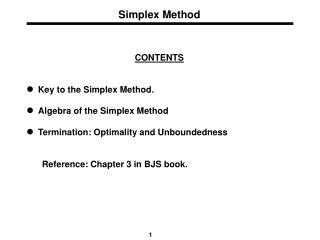
SIMPLEX METHOD FOR LP. LP Model. Preview of the Simplex Method. Developed by G B Dantzig in 1947. Similar to graphical method. The optimal solution lies at an extreme corner point of the multi-dimensional figure.

SIMPLEX METHOD FOR LP
E N D
Presentation Transcript
SIMPLEX METHOD FOR LP LP Model
Preview of the Simplex Method • Developed by G B Dantzig in 1947. • Similar to graphical method. • The optimal solution lies at an extreme corner point of the multi-dimensional figure. • Simplex method examines the extreme points in a systematic manner, till we reach optimal solution. • Hence iterative in nature. SIMPLEX METHOD
Gauss Jordan Elimination Method • A LP in standard form has both decision variables and slack variables. • Both are admissible variables. • If there are m constarint equations and n admissible variables then • if m = n then a unique solution exists. • if m > n then m-n equations have to be linearly dependent. • if m < n then optimization is required. SIMPLEX METHOD
Standard LP Model • The Standard LP Model shall have following characteristics: • All the constraints should be expressed as equations by adding slack or surplus and or artificial variables. • The right hand side of each constraint should be made non-negative, if is not, then this should be made by multiplying both sides by –1. • The objective function may be maximisation type or minimisation type. • An LP is in “canonical form” if it is written so that it is in standard form, and such that each constraint has a variable with a coefficient “1” and such that that variable has a 0 in all other constraints. SIMPLEX METHOD
SIMPLEX METHOD ISSUES • Major Issues of the Simplex Algorithm • How does one get the LP into the correct starting form? • How does one recognize optimality and unboundedness? • How does one move to the next corner point solution SIMPLEX METHOD
Slack Variables • Slack Variable – For constraints of type , the RHS normally represents the limit on the availability of a resource, and the LHS represents the usage of this resource by different activities. Slack represents amount of resource exceeding its usage • 6x1 + 4 x2 24 is converted to following by adding slack. • 6x1 + 4 x2 + s1 = 24 SIMPLEX METHOD
Surplus Variables • Constraints of type normally set minimum specification requirements. In this case the surplus represents the excess of the LHS over the minimum requirement. • For example x1 + x2 800 is mathematically equivalent to • x1 + x2 –S1 = 800 SIMPLEX METHOD
Unrestricted Variables • In some cases of LP the variables may assume any real value. An unrestricted variable can then be expressed in terms of two non-negative variables by using the substitution • x j = x j+ - x j- where x j+, x j- are non negative. SIMPLEX METHOD
Example • Express the following in standard LP Model form • Maximise z = 2x1 + 3x2 + 5x3 • subject to • x1 + x2 – x3 -5 • -6x1 + 7x2 –9x3 4 • x1 + x2 + 4 x3 = 10 • x1, x2 0 • x3 unrestricted SIMPLEX METHOD
Solution • The first constraint has a negative RHS, which needs to be converted to positive by multiplying both sides by –1. • After this the equality becomes < type and hence we have to add a slack variable to first equation. • Add slack s2 to second constraint • No change in third equation. • Substitute unrestricted x3 = x3+ - x3- in the objective and all constraints. x3+ & x3- > 0. • -x1 – x2 + x3+ - x3- + s1 = 5 SIMPLEX METHOD
Standard Form • Maximise z = 2x1 + 3x2 + 5x3+ - 5x3- • Subject to -x1 – x2 + x3+ - x3- + s1 = 5 - 6x1 + 7x2 - 9x3+ + 9x3- + s2 = 4 x1 + x2 + 4x3+ - 4x3- = 10 x1, x2, x3+ & x3- , s1, s2 0 SIMPLEX METHOD
STEPS IN SIMPLEX • Formulation of the mathematical model. • Introduction of slack, surplus and artificial variable. • Set up initial solution. • Look for the basis matrix whose only principal diagonal elements are present. • Test for optimality • Select entering variable • Select the leaving variable. • Finding new solution • Repeat the procedure SIMPLEX METHOD
Testing for Optimality • Calculate cj-zj for all non-basic variables. • To obtain value of zj, multiply each element under (column aj of coefficient matrix) with corresponding element (coefficient of basic variables). • Examine value of cj – zj. • The possible solutions are • If all cj – zj are 0, then the BFS is optimal. • If at least one column of the coefficient matrix (ak) for which ck – zk >0 and all elements are negative (aik<0), then there exists an unbounded solution to the given problem. • If at least one cj – zj > 0 and each of these has at least one positive element (ajk) for some row, then it indicates that an improvement in the value of objective function Z is possible. SIMPLEX METHOD
Test for Entering & Leaving Variable • In case of step III of optimality test, then select the variable that has the largest cj-zj value to enter into the solution. • ck – zk = Max {(cj-zj); cj-zj >0} • Column to be entered is called key or pivot column • Test for leaving variable – The basic variable that leaves shall be the one which reaches zero early when the entering variable is increased. • Mathematically the replacement ratio is selected as the minimum non-negative ratio of solution variable divided by the key column element. SIMPLEX METHOD
Finding new Solution • Deploy Gauss Elimination method to make the key element as 1. • Other elements of the key column, other than key element, are eliminated. • We will again get a canonical form LP with new basic variable included. • Again test the new solution for optimality and repeat till optimal solution is reached. SIMPLEX METHOD
EXAMPLE SIMPLEX METHOD
INITIAL STEPS SIMPLEX METHOD
Check for Optimality entering variable leaving variable Since all cj – zj > 0, j = 1, 2 &3, the current solution is not optimal SIMPLEX METHOD
Entering & Leaving Variable Variable x2 is chosen as entering variable as c2 – z2 is the largest positive number. The value of z will increase by 5 for every unit of x2. Thus contribution of x2 is more. Thus x2 is the key column. The leaving variable is chosen based on the minimum ratio as discussed. This means that as x2 is increased which variable approaches zero very fast. We see that s1 is minimum and hence leaving variable is s1 SIMPLEX METHOD
Finding New Rows SIMPLEX METHOD
New Tableau We see from above table that the new entering variable is x3 and the leaving variable is s2. We repeat the iterations SIMPLEX METHOD
Next Iteration SIMPLEX METHOD
Next Iteration SIMPLEX METHOD
Check for Optimality • Notice that all cj – zj are zero. • Hence the optimal solution is reached. • The optimal value of z is 18.659 • The values of decision variables are • x1 = 2.171 • x2 = 1.22 • x3 = 1.522 SIMPLEX METHOD
Basic Feasible Solution • Every basic feasible solution of a linear program in standard form is a corner point solution, and vice versa SIMPLEX METHOD
Simplex Steps ( Max Problem) • Step 0. The problem is in canonical form and bj ≥0. • Step 1. If cj – zj < 0 then stop. The solution is optimal. • Step 2. Choose any non-basic variable to pivot in with cj-zj > 0, e.g., ck – zk = max { (cj –zj); cj – zj > 0 }. If aik≤0 for all i, then stop; the LP is unbounded. • Step 3. Pivot out the basic variable in row r, where r is chosen by the min ratio rule, that is r = min(xbi/arj:arj> 0 ). • Step 4. Replace the basic variable in row r with variable xr and re-establish canonical form (i.e., pivot on the coefficient ) • Step 5. Go to Step 1. SIMPLEX METHOD

