Download
1 / 52
520 likes | 554 Vues
Discover the stochastic and recurrent nature of Boltzmann Machines, a type of neural network that mimics simulated annealing. Learn how they solve complex combinatorial problems, model data, and use distributed representations. Explore the training, units, and dynamics of Boltzmann Machines.

E N D
Maszyny Boltzmanna Inteligentne Systemy Autonomiczne W oparciu o wyklad Prof. Geoffrey Hinton University of Toronto and http://en.wikipedia.org/wiki/Boltzmann_machine oraz Prof. Włodzisława Ducha Uniwersytet Mikołaja Kopernika Janusz A. Starzyk Wyzsza Szkola Informatyki i Zarzadzania w Rzeszowie
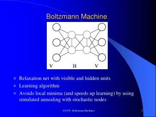
Maszyna Boltzmanna • Maszyna Boltzmana jest typemstochastycznej rekurencyjnej sieci neuronowejsymulowanego wyżarzania. • Maszyny Boltzmana można traktować jako stochastyczny, generujący odpowiednik sieci Hopfielda. • Maszyna Boltzmana jest siecią jednostek mających jednostki „energii”, które są binarnie stochastyczne. • Były one jednymi z pierwszych przykładów sieci neuronowej zdolnej do uczenia wewnętrznych reprezentacji i są w stanie rozwiązywać trudne problemy kombinatoryczne.
Maszyna Boltzmana • Stochastyczna siec atraktorowa • Podobna do modelu Hopfielda • Binarne neurony • Symetryczne połączenia • Ukryte neurony. • Asynchroniczna dynamika. • Neurony stochastyczne i stopniowe chłodzenie: Wyjścia Wejścia
Działanie Maszyn Boltzmana • Uczenie: sieć modeluje środowisko.Znaleźć zbiór wag pozwalających odtworzyć obserwowane częstości sygnałów wejściowych- model maksymalnego prawdopodobieństwa. • Założenia: • sygnały wejściowe wolnozmienne • sieć dochodzi do równowagi • brak korelacji pomiędzy strukturami danych wejściowych: prawdopodobienstwo p+(Va) każdego z 2n wektorów binarnych wystarczy. • Różnice między działaniem swobodnym i wymuszonym pozwalają obliczyć korelacje wzbudzeń neuronów i pożądaną zmianę wag:
Zajmowanie się strukturami złożonymi • Rozważ zestaw danych, w którym każdy obraz zawiera N różnych rzeczy: • Rozproszona reprezentacja wymaga pewnej liczby neuronów, która jest liniową funkcją N. • Lokalna reprezentacja (np. model mieszany) wymaga liczby neuronów, która jest wykładniczą funkcją N. • „Mieszanki” wymagają jeden model dla każdej możliwej kombinacji. • Reprezentacje rozproszone są generalnie trudniejsze w dopasowaniu do danych, ale są jedynym sensownym rozwiązaniem. • Maszyny Boltzmana wykorzystują reprezentacje rozproszone do modelowania binarnych danych.
Jednostki stochastyczne • Zastąp binarne jednostki progowe przez jednostki stochastyczne, które podejmują przypadkowe decyzje. • Temperatura kontroluje poziom szumu. • Prawdopodobieństwo włączenia jednostek wynosi: temperatura
Jak maszyny Boltzmana modelują dane? • To nie jest przyczynowymodel generatywny(jak model mieszany) w którym najpierwwybieramy stany ukryte a następnie wybieramy stany widoczne przy tych stanach ukrytych. • Zamiast tego, wszystko jest zdefiniowane poprzez energie konfiguracjiłącznych jednostekwidzialnych i ukrytych. • Jednostki widzialne V są tymi, które otrzymują informację ze „środowiska”, np. zbiór treningowy jest grupą wektorów binarnych okreslonych na zbiorze V
Energia konfiguracjiłącznej binarny stan jednostkii w konfiguracji łącznej alfa, beta waga pomiędzy i oraz j progi Energia z konfiguracją alfa w widzialnych jednostkach i beta w niewidzialnych. indeksy wszystkich roznych par i oraz j
Prawdopodobieństwo konfiguracji łącznej jednostekwidzialnych i ukrytych zależy od energii tej konfiguracji łącznej w porównaniu z energiami wszystkich innych konfiguracjiłącznych. Prawdopodobieństwo konfiguracji widzialnychjednostek jest sumą prawdopodobieństw wszystkichkonfiguracji łącznych, które je zawierają. Wykorzystanie energii do zdefiniowania prawdopodobieństwa funkcja podziału konfig. alfa na widzialnych jednostkach
Wykorzystanie energii do zdefiniowania prawdopodobieństwa • Naszym celem jest aproksymacja „realnego" rozkładup(v) wykorzystującp(v,h) dostarczane (ewentualnie) przez maszynę. • Aby określićpodobieństwodwóch rozkładów wykorzystujemy odległość Kullback-Leiblerga, • Są dwie fazy trenowania maszyny. • Faza „Pozytywna”jest gdy stany jednostekwidzialnych są przypisane do konkretnego binarnego wektora stanu pobranego ze zbioru treningowego. • Faza „Negatywna” występuje gdy żadne jednostki nie mają stanów zdeterminowanych przez dane zewnętrzne.
Wykorzystanie energii do zdefiniowania prawdopodobieństwa • Gradient odległości G w stosunku do danej wagi, wij, jest przedstawiony za pomocą bardzo prostego równania: • jest prawdopodobieństwem ze obie jednostki i oraz j, sa aktywne gdy maszyna jest w równowadze w faziepozytywnej. • jest prawdopodobieństwem ze obie jednostki i oraz j, sa aktywne gdy maszyna jest w równowadze w fazienegatywnej.
Wykorzystanie energii do zdefiniowania prawdopodobieństwa • W równowadze cieplnej prawdopodobieństwo dowolnego globalnego stanu s gdy sieć działa swobodnie jest dane przez rozkład Boltzmana (stąd nazwa „Maszyna Boltzmana”). • Ta reguła uczenia się jest biologicznie wiarygodna ponieważ wykorzystuje tylko „lokalne” informacje. • Aby zaistnieć, połączenie potrzebuje tylko informacji o dwóch łączonych neuronach.
A B C Sieci zaszumione znajdują lepsze minima energii • Sieć Hopfielda zawsze wykonuje decyzje, które redukują energię. • To uniemożliwia wyjsciez lokalnego minimum. • Możemy użyć przypadkowego szumu aby uniknąć mało znaczącego minimum. - Wystartowanie z dużym poziomem szumu ułatwia przekroczyć bariery energii. • Powolna redukcja szumu pozostawia system w głębokim minimum -To jest „symulowane wyżarzanie”
-1 h1 h2 +2 +1 v1 v2 Przykład jak wagi definiują rozkład. 1 1 1 1 2 7.39 .186 1 1 1 0 2 7.39 .186 1 1 0 1 1 2.72 .069 1 1 0 0 0 1 18.5 .025 1 0 1 1 1 2.72 .069 1 0 1 0 2 7.39 .186 1 0 0 1 0 1 .025 1 0 0 0 0 1 12.11 .025 0 1 1 1 0 1 .025 0 1 1 0 0 1 .025 0 1 0 1 1 2.72 .069 0 1 0 0 0 1 5.72 .025 0 0 1 1 -1 0.37 .009 0 0 1 0 0 1 .025 0 0 0 1 0 1 .025 0 0 0 0 0 1 3.37 .025 suma =39.70 0.466 0.305 0.144 0.084
Uzyskanie próbki z modelu. • Jeśli jest więcej niż kilka ukrytych jednostek, używamy metodę Monte Carlo łańcuchów Markowa (ang. Markov Chain Monte Carlo, MCMC) aby uzyskać próbki z modelu: • Zacznij w przypadkowej konfiguracji globalnej. • Wybieraj jednostki przypadkowo, dopuszczając do stochastycznego uaktualnienia ich stanów w oparciu o przyrosty energii (ang. energy gap) • Użyj symulowanego wyżarzania by zredukować czas potrzebny do otrzymania równowagi cieplnej. • W równowadze cieplnej, prawdopodobieństwo konfiguracji globalnej jest określone rozkładem Boltzmana.
Cel nauki • Maksymalizacja wyniku prawdopodobieństwa, które maszyna Boltzmana przypisuje do wektorów w zbiorze treningowym. • Jest to równoznaczne z maksymalizacją sumy logarytmów prawdopodobieństw wektorów treningowych . • Jest to również równoznaczne z maksymalizacją prawdopodobieństw, że zaobserwujemy te wektory w jednostkach widzialnych jeśli weźmiemy przypadkowe próbki po uzyskaniu przez całą sieć równowagi cieplnej bez udziału sygnału zewnętrznego.
Bardzo dziwny wynik • Wszystko co jedna waga musi wiedzieć o innych wagach i o danych jest zawarte w różnicy dwóch korelacji. wartość oczekiwana iloczynu stanów w równowadze cieplnej gdy wektor treningowy jest ‘wymuszony’ na jednostkach widocznych wartość oczekiwana iloczynu stanów w równowadze cieplnej gdy nic nie jest ‘wymuszone’ Pochodna logarytmu prawdopodob. jednego wektora treningowego
Wsadowy algorytm uczenia. • Faza pozytywna • Wymuś wektor danych na jednostkach widocznych. • Pozwól jednostkom ukrytym uzyskać równowagę cieplną o temperaturze 1 (można użyć wyżarzania, by to przyspieszyć) • Policz dla wszystkich par jednostek • Powtórz dla wszystkich wektorów danych w zbiorze treningowym • Faza negatywna • Nie wymuszaj żadnej z jednostek • Pozwól całej sieci osiągnąć równowagę cieplną o temperaturze 1 (gdzie zaczynamy?) • Policz dla wszystkich par jednostek. • Powtórz wielokrotnie aby dobrze oszacować wyniki • Aktualizacja wag • Uaktualnij każdą wagę proporcjonalnie do różnicy w w dwóch fazach
Ograniczone Maszyny Boltzmana (ang. Restricted Boltzmann Machines) • Ograniczamy spójność aby ułatwić wnioskowanie i uczenie. • Tylko jedna warstwa jednostek ukrytych. • Brak połączeń między jednostkami ukrytymi. • W RBM wystarczy jeden krok aby uzyskać równowagę cieplną gdy jednostki widzialne są ‘wymuszone’. • Możemy więc szybko otrzymać dokładną wartość : j ukryte widoczne i
Algorytm uczenia ograniczonejmaszyny Boltzmana Zacznij od wektora treningowego na jednostkach widocznych. Uaktualnij równolegle wszystkie jednostki ukryte. Uaktualnij równolegle wszystkie jednostki widoczne by uzyskać „rekonstrukcję” Uaktualnij jednostki ukryte jeszcze raz. j j i i t = 0 t = 1 rekonstrukcja dane Nie postępuje to z gradientem logarytmu prawdopodobieństwa (likelihood). Ale funkcjonuje bardzo dobrze.
Boltzmann Machines Pelna wersja
Modeling binary data • Given a training set of binary vectors, fit a model that will assign a probability to other binary vectors. • Useful for deciding if other binary vectors come from the same distribution. • This can be used for monitoring complex systems to detect unusual behavior. • If we have models of several different distributions it can be used to compute the posterior probability that a particular distribution produced the observed data.
Limitations of mixture models • Mixture models assume that the whole of each data vector was generated by exactly one of the models in the mixture. • This makes is easy to compute the posterior distribution over models when given a data vector. • But it cannot deal with data in which there are several things going on at once. mixture of 10 models mixture of 100 models
Boltzmann Machine • A Boltzmann machine is the name given to a type of simulated annealing stochastic recurrent neural network by Geoffrey Hinton and Terry Sejnowski. • Boltzmann machines can be seen as the stochastic, generative counterpart of Hopfield nets. • Boltzmann machine is a network of units with an "energy" units are binary stochastic. • They were one of the first examples of a neural network capable of learning internal representations, and are able to represent and (given sufficient time) solve difficult combinatoric problems.
Maszyna Boltzmana • Stochastyczna siec atraktorowa • Podobna do modelu Hopfielda • Binarne neurony • Symetryczne połączenia • Ukryte neurony. • Asynchroniczna dynamika. • Neurony stochastyczne i stopniowe chłodzenie: Wyjścia Wejścia
Dzialanie Maszyn Boltzmana • Uczenie: sieć modeluje środowisko.Znaleźć zbiór wag pozwalających odtworzyć obserwowane częstości sygnałów wejściowych- model maksymalnego prawdopodobieństwa. • Założenia: • sygnały wejściowe wolnozmienne • sieć dochodzi do równowagi • brak korelacji pomiędzy strukturami danych wejściowych: prawdopodobienstwo p+(Va) każdego z 2n wektorów binarnych wystarczy. • Różnice między działaniem swobodnym i wymuszonym pozwalają obliczyć korelacje wzbudzeń neuronów i pożądaną zmianę wag:
Dealing with compositional structure • Consider a dataset in which each image contains N different things: • A distributed representation requires a number of neurons that is linear in N. • A localist representation (i.e. a mixture model) requires a number of neurons that is exponential in N. • Mixtures require one model for each possible combination. • Distributed representations are generally much harder to fit to data, but they are the only reasonable solution. • Boltzmann machines use distributed representations to model binary data.
Stochastic units • Replace the binary threshold units by binary stochastic units that make biased random decisions. • The temperature controls the amount of noise. • Decreasing all the energy gaps between configurations is equivalent to raising the noise level. • The probability of a unit being on is given by: temperature
How a Boltzmann Machine models data • It is not a causal generative model (like a mixture model) in which we first pick the hidden states and then pick the visible states given the hidden ones. • Instead, everything is defined in terms of energies of joint configurations of the visible and hidden units. • The visible units V are those which receive information from the "environment", i.e. the training set is a bunch of binary vectors over the set V
The Energy of a joint configuration binary state of unit i in joint configuration alpha, beta weight between units i and j bias of unit i Energy with configuration alpha on the visible units and beta on the hidden units indexes every non-identical pair of i and j once
The probability of a joint configuration over both visible and hidden units depends on the energy of that joint configuration compared with the energy of all other joint configurations. The probability of a configuration of the visible units is the sum of the probabilities of all the joint configurations that contain it. Using energies to define probabilities partition function configuration alpha on the visible units
Using energies to define probabilities • Our goal is to approximate the "real" distribution p(v) using the p(v,h) produced (eventually) by the machine. • To measure how similar the two distributions are we use the Kullback-Leibler distance, G: • There are two phases of machine training. • “Positive" phase is where the visible units' states are set to a particular binary state vector sampled from the training set. • “Negative" phase where no units have their state determined by external data.
Using energies to define probabilities • The gradientof G with respect to a given weight, wij, is given by the very simple equation: • is the probability of units i and j both being on when the machine is at equilibrium on the positive phase. • is the probability of units i and j both being on when the machine is at equilibrium on the negative phase.
Using energies to define probabilities • This result follows from the fact that at the thermal equilibrium the probability of any global state s when the network is free-running is given by the Boltzmann distribution (hence the name "Boltzmann machine"). • This learning rule is biologically plausible because the only information needed to change the weights is provided by "local" information. • That is, the connection (or biological synapse) needs only information about the two neurons it connects.
Noisy networks find better energy minima • A Hopfield net always makes decisions that reduce the energy. • This makes it impossible to escape from local minima. • We can use random noise to escape from poor minima. • Start with a lot of noise so its easy to cross energy barriers. • Slowly reduce the noise so that the system ends up in a deep minimum. This is “simulated annealing”. • We will come back to simulated annealing later. For now, we will keep the noise level fixed to avoid unnecessary complications in explaining the other good things that result from using stochastic units. A B C
-1 h1 h2 +2 +1 v1 v2 An example of how weights define a distribution 1 1 1 1 2 7.39 .186 1 1 1 0 2 7.39 .186 1 1 0 1 1 2.72 .069 1 1 0 0 0 1 18.5 .025 1 0 1 1 1 2.72 .069 1 0 1 0 2 7.39 .186 1 0 0 1 0 1 .025 1 0 0 0 0 1 12.11 .025 0 1 1 1 0 1 .025 0 1 1 0 0 1 .025 0 1 0 1 1 2.72 .069 0 1 0 0 0 1 5.72 .025 0 0 1 1 -1 0.37 .009 0 0 1 0 0 1 .025 0 0 0 1 0 1 .025 0 0 0 0 0 1 3.37 .025 total =39.70 0.466 0.305 0.144 0.084
Getting a sample from the model • If there are more than a few hidden units, we cannot compute the normalizing term (the partition function) because it has exponentially many terms. • So use Markov Chain Monte Carlo (MCMC) to get samples from the model: • Start at a random global configuration • Keep picking units at random and allowing them to stochastically update their states based on their energy gaps. • Use simulated annealing to reduce the time required to approach thermal equilibrium. • At thermal equilibrium, the probability of a global configuration is given by the Boltzmann distribution.
Getting a sample from the posterior distribution • The number of possible hidden configurations is exponential so we need MCMC to sample from the posterior over distributed representationsfor a given data vector. • MCMC is just the same as getting a sample from the model, except that we keep the visible units clamped to the given data vector. • Only the hidden units are allowed to change states • Samples from the posterior are required for learning the weights.
The goal of learning • Maximize the product of the probabilities that the Boltzmann machine assigns to the vectors in the training set. • This is equivalent to maximizing the sum of the log probabilities of the training vectors. • It is also equivalent to maximizing the probabilities that we will observe those vectors on the visible units if we take random samples after the whole network has reached thermal equilibrium with no external input.
Why the learning could be difficult Consider a chain of units with visible units at the ends If the training set is (1,0) and (0,1) we want the product of all the weights to be negative. So to know how to change w1 or w5 we must know w3. w2 w3 w4 hidden visible w1 w5
A very surprising fact • Everything that one weight needs to know about the other weights and the data is contained in the difference of two correlations. Expected value of product of states at thermal equilibrium when the training vector is clamped on the visible units Expected value of product of states at thermal equilibrium when nothing is clamped Derivative of log probability of one training vector
The batch learning algorithm • Positive phase • Clamp a datavector on the visible units. • Let the hidden units reach thermal equilibrium at a temperature of 1 (may use annealing to speed this up) • Sample for all pairs of units • Repeat for all datavectors in the training set. • Negative phase • Do not clamp any of the units • Let the whole network reach thermal equilibrium at a temperature of 1 (where do we start?) • Sample for all pairs of units • Repeat many times to get good estimates • Weight updates • Update each weight by an amount proportional to the difference in in the two phases.
Why is the derivative so simple? • The probability of a global configuration at thermal equilibrium is an exponential function of its energy. • So settling to equilibrium makes the log probability a linear function of the energy • The energy is a linear function of the weights and states • The process of settling to thermal equilibrium propagates information about the weights.
The positive phase finds hidden configurations that work well with v and lowers their energies. The negative phase finds the joint configurations that are the best competitors and raises their energies. Why do we need the negative phase?
Restricted Boltzmann Machines • We restrict the connectivity to make inference and learning easier. • Only one layer of hidden units. • No connections between hidden units. • In an RBM it only takes one step to reach thermal equilibrium when the visible units are clamped. • So we can quickly get the exact value of : j hidden visible i
A picture of the Boltzmann machine learning algorithm for an RBM j j j j a fantasy i i i i t = 0 t = 1 t = 2 t = infinity Start with a training vector on the visible units. Then alternate between updating all the hidden units in parallel and updating all the visible units in parallel.
A surprising short-cut j j Start with a training vector on the visible units. Update all the hidden units in parallel Update the all the visible units in parallel to get a “reconstruction”. Update the hidden units again. i i t = 0 t = 1 reconstruction data This is not following the gradient of the log likelihood. But it works very well.
Why does the shortcut work? • If we start at the data, the Markov chain wanders away from them data and towards things that it likes more. We can see what direction it is wandering in after only a few steps. It’s a big waste of time to let it go all the way to equilibrium. • All we need to do is lower the probability of the “confabulations” it produces and raise the probability of the data. Then it will stop wandering away. • The learning cancels out once the confabulations and the data have the same distribution. • We need to worry about regions of the data-space that the model likes but which are very far from any data. • These regions cause the normalization term to be big and we cannot sense them if we use the shortcut.
Neurodynamika Spoczynkowa aktywność neuronów (1-5 impulsów/sek) Ok. 10.000 impulsów/sek dochodzi do neuronu w pobliżu progu. 1. Stabilna sieć z aktywnością spoczynkową: globalny atraktor. 2. Uczenie się przez tworzenie nowych atraktorów. Model Amit, Brunel 1995 Aktywność tła ma charakter stochastyczny. Jednorodność: neurony w identycznym środowisku. Impulsy wysyłane przez różne neurony nie są skorelowane. Aktywacja neuronu jest sumą wkładów synaptycznych.