Surface-Based Cross-Subject Analysis
Surface-Based Cross-Subject Analysis. SSCC/NIMH/NIH/DHHS/USA/Earth. Geometry and Topology. Geometry: Spatial location X,Y,Z coordinates of brain structures Topology: Spatial connectivity Relative positions of brain structures along the surface.

Surface-Based Cross-Subject Analysis
E N D
Presentation Transcript
Surface-Based Cross-Subject Analysis SSCC/NIMH/NIH/DHHS/USA/Earth
Geometry and Topology • Geometry: Spatial location • X,Y,Z coordinates of brain structures • Topology: Spatial connectivity • Relative positions of brain structures along the surface • Geometric proximity does not imply topological proximity • If you care about the topology of activation, you should transfer FMRI data onto the surface before spatial manipulations of the data
Group analysis • Group analysis requires data defined over a domain common to all subjects • Talairach space for volume-based analysis + Small amount of geometric distortion • No respect for topology of activation • Spherical coordinate system for surface-based analysis + Preserves the topology of activation • Considerable geometric distortion • Preserving the topology of activation is Good in general and crucial for • Retinotopy • Plasticity • High-resolution Mapping
Surface domain • Surface models are modeled using a set of interconnected nodes • Data are mapped to the nodes forming the mesh • Surface models from different subjects have different meshes (i.e. surfaces are not isotopic) and differing geometries • Cross-subject analysis requires warping the surfaces to match a common domain • A domain defined by a tessellated sphere and a spherical coordinate system has been adopted by Caret/SureFit [Van Essen et al. 1997, 1998 ] and FreeSurfer [Fischl et al. 1999]
Spherical Warping Surface-based warping is more accurate than the more common Talairach volume-based analysis because it preserves the topology of the cortical sheet and uses more landmarks for the warping
Mapping data Problem is that surfaces from different subjects are not topologically isomorphic (different meshes). Data from each subject are mapped onto the icosahedral surface for group analysis Cumbersome and unnecessary interpolation n1 n2 n3
Our twist Instead of interpolating data values to the icosahedral nodes, interpolate using the coordinates of the original surface’s node. This results in a surface that is virtually identical in geometry to the original surface but with the mesh of the icosahedron. Cross-subject surface based analysis is thus reduced to node-based analysis
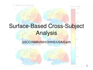
Standard meshes for 6 subjects • 6 standard-mesh surface models from different subjects. • Node colors encode for node index n on the standard mesh. • Nodes with similar indices correspond to comparable sulcal landmarks despite anatomical variability across subjects.
Original-mesh versions of the standard-mesh surfaces with the same coloration schemes • Because these surfaces have differing numbers of nodes, some colors may not be represented • Nodes with similar indices no longer correspond to comparable anatomical areas • Small clusters of red color show regions where new nodes were later added to correct topological errors of the surface
SUMA demo • cd std_meshes • suma –spec All_lh_ld141.spec & • Open multiple viewers (ctrl+n) • Lock all viewers together (ctrl+u, Lock All v) • Turn off background (‘b’) • Switch each viewer to a different state • surfaces from different subjects are assigned different states • This is a workaround lacking style. Will fix it later. • Click in one view and watch the cross hair jump to corresponding locations in other views • Anatomical location should match, within the warping tolerance • Load the color file lh_ld141_smoothcol2.1D.col (ctrl+c) • This is the color file used to create the figures on the previous slides
Implications • Greatly simplifies: • cross-subject analysis in the surface domain • data exchange between groups using the same/similar templates • data management and mapping from atlases (within/across species) • What templates to use then? • function based • sulcal patterns • automated segmentation
Creating standard-mesh surfaces • Required Data: • Original Surface models • Warped Spherical surface • Spec file of the surfaces above (i.e. lh.spec) • Creating the standard-mesh versions of the original surfaces MapIcosahedron -spec lh.spec \ Written by Brenna Argall -ld 141 \ -prefix ld141 -spec SpecFile: option specifying spec file with original surfaces -ld n : number of subdivisions for each edge of the icosahedron. Nv = 2 + 10n2 (198812 vertices) Nt = 20n2 (397620 triangles) Ne = 30n2 (596430 edges) -prefix: prefix assigned to standard mesh surfaces
Creating standard-mesh surfaces • The whole process takes 6 minutes on a 1.2 Ghz computer running linux • You can compare original and standard surfaces using: • SUMA • create a spec file containing both original and standard-mesh surfaces. • open two views, one showing original surface and one showing standard-mesh surfaces • link viewers by coordinates (not by node index) from the SUMA controller (ctrl+u) • CompareSurfaces Written by Shruti Japee • a program that calculates the distance from each node on surface 1 along its normal to surface 2 • SurfaceMetrics • a program that calculates metrics of the mesh like edge lengths, triangle areas, curvature, etc.
Mapping data As done with SUMA, but now using standard meshes
Mapping Options • Shell/volume Intersection • Surface/volume Intersection
Mapping options • Shell/volume Intersection • Multiple voxels possible per node • Surface/volume Intersection • One voxel per node
Mapping data: Volume Surface • Use 3dVol2Surf to map individual subject data onto each surface • Example: Mapping functional data onto surface, with thresholding 3dVol2Surf -spec lh.spec \ -sv SurfVol_AlndExp+orig \ -grid_parent DataVol+orig \ -cmask '-a DataVol+orig[3] -expr step(a-72)' \ -map_func ave \ -oom_value -999.9 \ -out_1D DataSurf.1D.dset Written by Rick Reynolds • -spec: SUMA spec file containing surface(s) to be used in mapping. 3dVol2Surf uses one or two surfaces for the mapping. Surfaces must have MappingRef = SAME • -sv: Surface Volume used to align surface to data • -grid_parent: AFNI volume containing data to be mapped. DataVol contains 4 sub-bricks with the last one being the threshold. • -cmask: Option for masking data in DataVol. Threshold value was 72 • -map_func: Method for handling multiple voxel to one node mapping • -oom_value -999.9 : Assign -999.9 to nodes that fall in inactivated voxels • -out_1D: Output file • Use –help option for detailed help (~500 lines)
1D files as data sets • Most 3dSomething command line programs can read 1D instead of volumetric data • The "spatial" direction is down the columns (vertical). • The default is that across the rows (horizontal) is a "bucket" dimension. • The new environment variable AFNI_1D_TIME, if set to YES, will cause the horizontal direction to be the time axis (with TR=1). • This makes it possible to input .1D files to programs that process 3D+time datasets • Some files need to be transposed first -- so that the time axis is horizontal rather than vertical. For example, assume fred.1D is a time series stored in a column vector. 1dtranspose fred.1D fred_q.1D 3dFourier -prefix fred_filt_q -highpass 0.1 -retrend fred_q.1D 1dtranspose fred_filt_q.1D fred_filt.1D rm -f fred_q.1D fred_file_q.1D
Sample output, the 1D format # -------------------------------------------------- # surface 'lh_mappedSmWm.asc', 'ave' : # # node 1dindex i j k vals v0 # ------ ------- --- --- --- ---- -------- 3 31978 42 51 7 2 -18.80515 64 30633 41 30 7 1 13.49998 7255 43375 47 37 10 2 11.25401 7256 43375 47 37 10 1 11.70573 7257 43375 47 37 10 2 11.25401 7317 39144 40 35 9 2 14.67585 7318 39145 41 35 9 2 17.08102 7358 47406 46 36 11 1 15.62297 7359 47406 46 36 11 1 15.62297 7435 30633 41 30 7 1 13.49998 (I omitted from the table above all nodes that had no values mapped to them. Such nodes will have v0 = -999.9 ) • Node: Surface node index • 1dindex: AFNI 1D Index of voxel mapped to node. In cases where multiple voxels contribute to 1 node, the first voxel is listed • i, j, k: AFNI indices of voxel mapped to node (3D version of 1dindex) • vals: Number of voxels mapped to node • v0: Value mapped to node. Here we mapped values from one sub-brick. If you map N sub-bricks you'll have v0 .. vN-1 columns.
Colorizing the mapping (the olde way) • At first you had to colorize a data set before viewing it in SUMA. • Now that is done interactively from SUMA’s ‘Surface Controller’. • ScaleToMap is used to show the mapped data in SUMA ScaleToMap -input DataSurf.1D.dset 0 6 \ -cmap RGYBR20 \ -msk -998 -1000 \ > DataSurf.1D.col • -input DataFile icol vcol: Node data file followed by column indices for node index and data • -cmap MapType: Type of colormap • -msk msk0 msk1: Range of values to exclude from color map • > DataSurf.1D.col : redirection of output to file (screen is the default). Output contains 4 columns: node index, R, G, B • DataSurf.1D.col can be loaded into SUMA using 'c' option # index R G B 3 0.000 0.862127 0.137873 64 1.000000 0.800135 0.000000 7255 1.000000 0.943492 0.000000
A simple cross-subject analysis • Calculate the mean value at each node from 3 subjects: 1deval -a 'DataSurf_s1.1D.dset[6]' \ -b 'DataSurf_s2.1D.dset[6]' \ -c 'DataSurf_s3.1D.dset[6]' \ -expr '(a + b + c) / 3' \ -index 'DataSurf_s1.1D.dset[0]' \ > DataSurf_mean.1D.dset • 1deval works much like 3dcalc but with 1D files -index option allows the addition of an index column (node indices) to the output. DataSurf_mean.1D.dset will contain 2 columns: node index and mean value • Appreciate why we forced an output for all node indices • Things to be careful about: • 1D files do not explicitly encode domain information • Up to you to make sure that the i th entry in all 1D files corresponds to the same node. • You must have the same number of values in all files
Things to lose some sleep over • When mapping data from volume to surface domains • If mapping assigns multiple voxels to one node • How do you deal with functional data sets? • Do you average statistics? • Do you apply a threshold before or after averaging? • What if some of the voxels are active and some are not? • These problems are best avoided by: • Mapping the time series data onto the surface • Performing statistical analysis directly in the surface domain using 3dSomething AFNI programs • When combining surface data across subjects • Same concerns as with volumetric group analysis • You can also create volumetric data from surface-based data • use 3dSurf2Vol, the reciprocal of 3dVol2Surf
Artifacts with standard meshes • At times, there are localized distortions between the standard-mesh surface and the original surface. • So far, these have all been caused by topological errors in the original spherical surfaces. • SurfQual was written to highlight these errors • if causing distortions, errors must be fixed with the program used to generate them. • These topological errors can be ignored if they do not cause any visible distortions in the standard-mesh surfaces.

