Network and Surface Analysis: Shortest Paths, Flow Dynamics, and Visualization Techniques
This lecture explores the fundamental concepts of network analysis, focusing on determining the shortest paths, cheapest routes, and maximum flow capacity within given networks. It also delves into surface analysis techniques, such as the use of contour maps and choropleth maps to visually represent various data, including elevation and distribution of resources. The discussion emphasizes the importance of accurate data classification, visualization challenges, and the relevance of advanced modeling techniques for robust surface and network analysis.

Network and Surface Analysis: Shortest Paths, Flow Dynamics, and Visualization Techniques
E N D
Presentation Transcript
Surface Analysis CS 128/ES 228 - Lecture 13a
Network Analysis • Given a network • What is the shortest path from s to t? • What is the cheapest route from s to t? • How much “flow” can we get through the network? • What is the shortest route visiting all points? Image from: http://www.eli.sdsu.edu/courses/fall96/cs660/notes/NetworkFlow/NetworkFlow.html#RTFToC2 CS 128/ES 228 - Lecture 13a
Network complexities All answers learned in CS 232! CS 128/ES 228 - Lecture 13a
When is an Elevation NOT an Elevation? • When it is rainfall, income, or any other scalar measurement • Bottom Line: It’s one more dimension (any dimension!) on top of the geographic data CS 128/ES 228 - Lecture 13a
Surface map • Contour map • Choroplethmap How do we display a map with “elevation”? CS 128/ES 228 - Lecture 13a
Choroplethmaps • Show areas of equal “elevation” in a uniform manner • Are usually “exact” approximations (through aggregation) • Subject to classification issues • Often intimately connected to queries CS 128/ES 228 - Lecture 13a
Simple uses of choropleths Ordinal • Population • Per capita income • Crop yield Categorical • Soil type • Political party control • Primary industry CS 128/ES 228 - Lecture 13a
Display issues for choropleths • Classification Type • Number of intervals • Colors CS 128/ES 228 - Lecture 13a
How do we select choroplethregions? • Based on existing polygons • Based on dissolved polygons • Based on nearest points CS 128/ES 228 - Lecture 13a
A Choroplethyou built CS 128/ES 228 - Lecture 13a
More complex queries using choropleths • Time series data • Population change • % of land in agricultural use • Computation driven • Total spending power = Average income x population • Average wheat yield = Total yield / Acreage of farms CS 128/ES 228 - Lecture 13a
Basic model for “computed choropleths” • Create new attribute data (usually within attribute table; sometimes with selection layer) • Set the display to key off that new data • Choose remaining display options CS 128/ES 228 - Lecture 13a
A riddle (sans funny punch line) • What is the difference between a choroplethmap and a 2-D query such as “how many points are in this polygon”? A fine (boundary) line • In truth, it is a matter of style of output. CS 128/ES 228 - Lecture 13a
Review of surface approximation “dimensions” • Local vs. Gradual • Exact vs. Approximate • Gradual vs. Abrupt • Deterministic vs. Stochastic CS 128/ES 228 - Lecture 13a
Thiessen polygons • Local • Exact • Abrupt • Deterministic CS 128/ES 228 - Lecture 13a
More sophisticated surface generation (trend surface) Use a “least squares”-like technique to fit a surface to the data CS 128/ES 228 - Lecture 13a
Trend Surfaces • Global • Approximate (in most cases) • Gradual • Deterministic • Better quality obtained by using higher order surface, but takes longer CS 128/ES 228 - Lecture 13a
Inverse distance interpolation Value of a point is related to the sum of the values of all other points divided by their distance from the given point CS 128/ES 228 - Lecture 13a
Inverse distance • Global (but effectively local) • Approximate (but close to exact) • Gradual • Deterministic • Can use different functions, e.g. inverse distance squared CS 128/ES 228 - Lecture 13a
Spatial moving average • Global (but heavily local) • Approximate (but close to exact) • Gradual • Deterministic CS 128/ES 228 - Lecture 13a
“Realistic” surface modeling • Requires approximating • “Show the impression, not the data” • Often involves slope and aspect • Commonly used for shading maps CS 128/ES 228 - Lecture 13a
Building “shade” • Shaded maps intrinsically include a “camera” and a “direction” • For “perspective”, color is determined using the dot product (trigonometry alert) of the value of the normal (aspect) and the camera vector (line of sight) CS 128/ES 228 - Lecture 13a
Some shaded surfaces Image from: Burrough & McDonnell, Principles of Geographic Information Systems, p. 192 CS 128/ES 228 - Lecture 13a
Where has all the rainfall gone? Image from: Burrough & McDonnell, Principles of Geographic Information Systems, p. 194 CS 128/ES 228 - Lecture 13a
It’s not calculus • Much analysis is done through “cellular” computation • Conway’s game of Life is an example http://www.bitstorm.org/gameoflife/ • Use the gradient to move “cells” of water to show flow and/or flooding CS 128/ES 228 - Lecture 13a
More complex models • To compute the irradiance, I, use the following formula I = [cos0cos + sin0sincos(0-A)]S0 x exp(-T0/cos0) where S0 is the exatmospheric solar flux, 0 is the solar zenith angle, etc. CS 128/ES 228 - Lecture 13a
Thoughts on surface analysis • Surface analysis is handy, but requires • Moderately complex database queries, or • Moderately complex mathematics • Fortunately, much of this is “built-in” through wizards (e.g. buffer wizard) CS 128/ES 228 - Lecture 13a
Some thoughts on surface generation • “There are three kinds of lies: lies, damned lies and statistics” Benjamin Disraeli, popularized by Mark Twain • “Anyone can lie with statistics” Anonymous • “A picture can lie more effectively than words” Anonymous CS 128/ES 228 - Lecture 13a