Evolution of High-Performance Computing: From Mainframes to Supercomputers
Trace the history and advancements in HPC from mainframes to supercomputers, including notable systems like Jaguar, Roadrunner, and Tianhe-1A. Explore concepts such as Amdahl's Law, parallel efficiency, and the evolution of processor architecture and filesystems. Learn about our Cray XT6m system and its modular architecture. Discover the scheduling system and tools used for performance analysis in HPC environments.

Evolution of High-Performance Computing: From Mainframes to Supercomputers
E N D
Presentation Transcript
High Performance Computing Andy Neal CS451
HPC History • Origins in Math and Physics • Ballistics tables • Manhattan Project • Not a coincidence that the CSU datacenter is in the basement of Engineering E wing – old Physics/Math wing • FLOPS (Floating point operations per second) • Our primary measure, other operations are irrelevant
Timeline 60-70's Mainframes Seymour Cray CDC Burroughs UNIVAC DEC IBM HP
Timeline 80’s • Vector Processors • Designed for operations on data arrays rather than single elements, first in the 70’s , ended by the 90’s • Scalar Processors • Personal Computers brought commodity CPUs increased speed and decreased cost
Timeline 90’s • 90's-2000's Commodity components / Massively parallel systems • Beowulf clusters – NASA 1994 "A supercomputer is a device for turning compute-bound problems into I/O-bound problems.“ – Ken Batcher
Timeline 2000’s Jaguar – 2005/2009 Oak Ridge (224,256 CPU cores 1.75 petaflops) Our Cray's forefather
Timeline 2000’s Roadrunner – 2008 Los Alamos (13,824 CPU cores, 116,640 Cell cores = 1.7 petaflops)
Timeline 2010’s Tianhe-1A 2010 - NSC-China (3,211,264 GPU cores, 86,016 CPU cores = 4.7 Petaflops)
Caveat of massively Parallel computing • Amdahl's law A program can only speed up relative to the parallel portion. • Speedup Execution time for a single Processing Element / execution time for a given number of parallel PEs • Parallel efficiency Speedup / PEs
Our Cray XT6m Our Cray XT6m (1248 CPU cores, 12 teraflops) At installation cheapest cost to flops ratio ever built! Modular system Will allow for retrofit and expansion
Cray modular architecture Cabinets are installed in a 2-d X-Y mesh 1 cabinet contains 3 cages 1 cage contains 8 blades 1 blade contains 4 nodes 1 node contains 24 cores (12 core symmetric CPUs) Our 1,248 compute cores and all “overhead” nodes represent 2/3 of one cabinet…
Node types • Boot • Lustrefs • Login • Compute • 960 cores devoted to the batch queue • 288 cores devoted to interactive use • As a “mid-size” supercomputer (m model) our unit maxes at 13,000 cores…
Hypertransport Open standard Packet oriented Replacement for FSB Multiprocessor interconnect Common to AMD architecture (modified) Bus speeds up to 3.2Ghz DDR A major differentiation between systems like ours and common linux compute clusters (where interconnect happens at the ethernet level).
LustreFilesystem Open standard (owned by Sun/Oracle) True parallel file system Still requires interface nodes Functionally similar to ext4 Currently used by 15 of the 30 fastest HPC systems
Optimized compilers • Uses Cray, PGI, PathScale and GNU • The crap compilers are the only licensed versions we have installed, they are also notably faster (being used to the specific architecture) • Supports • C • C++ • Fortan • Java (kind of) • Python (soon)
Performance tools • Craypat • Command line performance analysis • Apprentice2 • X-window performance analsis • Require instrumented compilation • (Similar to gdb – which also runs here…) • Provides detailed analysis of runtime data, cache misses, bandwidth use, loop iterations, etc.
Running a job • Nodes are Linux derived (SUSE) • Compute nodes extremely stripped down, only accessible through aprun • Aprun syntax: • Aprun –n[cores] –d[threads] –N[PE per node] executable • (Batch mode requires additional PBS instructions in the file but still uses the aprun syntax to execute the binary)
Scheduling – levels • Interactive • Designed for building and testing, job will only run if the resources are immediately available • Batch • Designed for major computation, jobs are allocated in a priority system (normally, we are currently running one queue)
Scheduling - system • Node allocation • Other systems differ here but our Cray does not share nodes between jobs, goal is to provide maximum available resources to the currently running job • Compute node time slicing • The compute nodes do time slice, though it’s difficult to see that from operation as they are only running their own kernel and their current job
MPI Every PE runs the same binary + More traditional IPC model +IP-style architecture (supports multicast!) + Versatile (spans nodes, parallel IO!) + MPI code will translate between MPI compatible platforms - Steeper learning curve - Will only compile on MPI compatible platforms…
MPI #include <mpi.h> using namespace MPI; main(intargc,char *argv[]) { intmy_rank, nprocs; Init(argc,argv); my_rank=COMM_WORLD.Get_rank(); nprocs=COMM_WORLD.Get_size(); if (my_rank == 0) { ... } ... }
OpenMP Essentially pre-built multi-threading + Easier learning curve + Fantastic timer function + Closer to a logical fork operation + Runs on anything! - Limits execution to a single node - Difficult to tune - Not yet implemented on GPU based systems (oddly unless you’re running windows…)
OpenMP #include <omp.h> ... double wstart = omp_get_wtime(); #pragmaomp parallel { #pragmaomp for reduction(+:variable_name) for(inti=0;i<N;++i){ ... } } double wstop = omp_get_wtime(); cout << "Dot product time (wtime)" << fixed << wstop - wstart << endl;
MPI / OpenMP Hybridization • These are not mutually exclusive • The reason for –N, –n, and –d flags… • This allows for limiting the number of PEs used on a node, to optimize cache use and keep from overwhelming the interconnect • According to ORNL this is the key to fully utilizing the current Cray architecture • I just haven’t been able to make this work properly yet :) • My MPI codes have always been faster
Programming Pitfalls • A little inefficiency goes a long way… • Given the large number of iterations your code will likely be running in any minor efficiency fault can quickly become overwhelming. • CPU time Vs. Wall Clock time • Given that these systems have traditionally been “pay for your cycles” don’t instrument your code with CPU time, it returns a cumulative value, even in MPI!
Demo time! • Practices and pitfalls Watch your function calls and memory usage, malloc is your friend! Loading/writing data sets is a killer that via Amdahl’s law, if you can use parallel IO, do it! Synchronization / data dependency is not your friend, every time you will have idle PEs.
Future Trends “Turnkey” supercomputers GPUs APUs OpenDL CUDA PVM
Resources • Requesting access – ISTeC requires faculty sponsor http://istec.colostate.edu/istec_cray/ • CrayDocs http://docs.cray.com/cgi-bin/craydoc.cgi?mode=SiteMap;f=xt3_sitemap • NCSA tutorials http://www.citutor.org/login.php • MPI-Forum http://www.mpi-forum.org/ • Page for this presentation http://www.cs.colostate.edu/~neal/ • Cray slides used with permission