Bayesian Methods with Monte Carlo Markov Chains I
Bayesian Methods with Monte Carlo Markov Chains I. Henry Horng-Shing Lu Institute of Statistics National Chiao Tung University hslu@stat.nctu.edu.tw http://tigpbp.iis.sinica.edu.tw/courses.htm. Part 1 Introduction to Bayesian Methods. Bayes’ Theorem. Conditional Probability:

Bayesian Methods with Monte Carlo Markov Chains I
E N D
Presentation Transcript
Bayesian Methods with Monte Carlo Markov Chains I Henry Horng-Shing Lu Institute of Statistics National Chiao Tung University hslu@stat.nctu.edu.tw http://tigpbp.iis.sinica.edu.tw/courses.htm
Bayes’ Theorem • Conditional Probability: • One Derivation: • Alternative Derivation: • http://en.wikipedia.org/wiki/Bayes'_theorem
False Positive and Negative • Medical diagnosis: • Type I and II Errors: hypothesis testing in statistical inference • http://en.wikipedia.org/wiki/False_positive
Bayesian Inference (1) • False positives in a medical test • Test accuracy by conditional probabilities: P(Test Positive|Disease) = P(R|H1) = 1-β = 0.99 P(Test Negative|Normal) = P(A|H0) = 1-α = 0.95. • Prior probabilities: P(Disease) = P(H1) = 0.001 P(Normal) = P(H0) = 0.999.
Bayesian Inference (2) • Posterior probabilities by Bayes’ theorem:True Positive Probability = P(Disease|Test Positive) = P(H1|R) = False Positive Probability = P(Normal|Test Positive) = P(H0|R) = (1 − 0.019) = 0.981.
Bayesian Inference (3) • Equal Prior probabilities: P(Disease) = P(H1) = P(Normal) = P(H0) = 0.5. • Posterior probabilities by Bayes’ theorem:True Positive Probability = P(Disease|Test Positive) = P(H1|R) = = P(R|H1) = 1-β! • http://en.wikipedia.org/wiki/Bayesian_inference
Bayesian Inference (4) • In the courtroom: • P(Evidence of DNA Match | Guilty) = 1 and P(Evidence of DNA Match | Innocent) = 10-6. • Based on the evidence other than the DNA match, P(Guilty) = 0.3 and P(Innocent) = 0.7. • By the Bayes Theorem, P(Guilty | Evidence of DNA Match) = = 0.99999766667.
Naive Bayes Classifier • Naive Bayes Classifier is a simple probabilistic classifier based on applying Bayes’ theorem with strong (naive) independence assumptions. • http://en.wikipedia.org/wiki/Naive_Bayes_classifier
Naive Bayes Probabilistic Model (1) • The probability model for a classifier is a conditional model P(C|F1,…,Fn)where C is a dependent class variable and F1,…,Fn are several feature variables. • By Bayes’ theorem,
Naive Bayes Probabilistic Model (2) • Use repeated applications of the definition of conditional probability:P(C,F1,…Fn)=P(C) P(F1,..Fn|C) =P(C)P(F1|C)P(F2,..Fn|C,F1) =P(C)P(F1|C)P(F2|C,F1)P(F3,..,Fn|C,F1,F2)and so forth. • Assume that each Fi is conditionally independent of every other Fj for i≠j, this means that P(Fi|C,Fj)=P(Fi|C). • So P(C,F1,…Fn) can be expressed as .
Naive Bayes Probabilistic Model (3) • So P(C|F1,…,Fn) cab be expressed like where Z is constant if the values of the feature variables are known. • Constructing a classifier from the probability model:
Bayesian Spam Filtering (1) • Bayesian spam filtering, a form of e-mail filtering, is the process of using a Naive Bayes classifier to identify spam email. • References: http://en.wikipedia.org/wiki/Spam_%28e-mail%29http://en.wikipedia.org/wiki/Bayesian_spam_filteringhttp://www.gfi.com/whitepapers/why-bayesian-filtering.pdf
Bayesian Spam Filtering (2) • Probabilistic model: where {words} mean {certain words in spam emails}. • Particular words have particular probabilities of occurring in spam emails and in legitimate emails. For instance, most email users will frequently encounter the word “Viagra” in spam emails, but will seldom see it in other emails.
Bayesian Spam Filtering (3) • Before mails can be filtered using this method, the user needs to generate a database with words and tokens (such as the $ sign, IP addresses and domains, and so on), collected from a sample of spam mails and valid mails. • After generating, each word in the email contributes to the email's spam probability. This contribution is called the posterior probability and is computed using Bayes’ theorem. • Then, the email's spam probability is computed over all words in the email, and if the total exceeds a certain threshold (say 95%), the filter will mark the email as a spam.
Bayesian Network (1) • Bayesian network is compact representation of probability distributions via conditional independence • For example, a Bayesian network could represent the probabilistic relationships between diseases and symptoms • http://en.wikipedia.org/wiki/Bayesian_networkhttp://www.cs.ubc.ca/~murphyk/Bayes/bnintro.htmlhttp://www.cs.huji.ac.il/~nirf/Nips01-Tutorial/index.html
Cloudy Sprinkler Rain Wet Grass S R P(W | S,R) Data + Prior Information Learner T 1.0 0.0 T T F 0.1 0.9 F T 0.1 0.9 F 0.01 0.99 F Bayesian Network (2) • Conditional independencies & graphical language capture structure of many real-world distributions • Graph structure provides much insight into domain • Allows “knowledge discovery”
Cloudy S R P(W | S,R) Sprinkler Rain T T 1.0 0.0 T F 0.1 0.9 Wet Grass F T 0.1 0.9 F F 0.01 0.99 Bayesian Network (3) Qualitative part: Directed acyclic graph (DAG) • Nodes - random variables • Edges - direct influence Quantitative part: Set of conditional probability distributions Together: Define a unique distribution in a factored form
Burglary Earthquake Radio Alarm Call Inference • Posterior probabilities • Probability of any event given any evidence • Most likely explanation • Scenario that explains evidence • Rational decision making • Maximize expected utility • Value of Information • Effect of intervention Radio
Example 1 (1) Cloudy Rain Sprinkler Wet Grass
Example 1 (2) • By the chain rule of probability, the joint probability of all the nodes in the graph above is P(C, S, R, W) = P(C) * P(S|C) * P(R|C, S) * P(W|C, S, R). • By using conditional independence relationships, we can rewrite this as P(C, S, R, W) = P(C) * P(S|C) * P(R|C) * P(W|S, R)where we were allowed to simplify the third term because R is independent of S given its parent C, and the last term because W is independent of C given its parents S and R.
Example 1 (3) • Bayes theorem: the posterior probability of each explanation where is a normalizing constant, equal to the probability (likelihood) of the data.
Example 1 (4) • So we see that it is more likely that the grass is wet because it is raining: the likelihood ratio is 0.708/0.430 = 1.647.
Maximum Likelihood Estimates (MLEs) vs. Bayesian Methods • Binomial Experiments: http://www.math.tau.ac.il/~nin/Courses/ML04/ml2.ppt • More Explanations and Examples: http://www.dina.dk/phd/s/s6/learning2.pdf
MLE (1) • Binomial Experiments: suppose we toss coin N times and the random variable is • We denote by the (unknown) probability P(Head). Estimation task: • Given a sequence of toss samples x1, x2,…, xN we want to estimate the probabilities P(H)= and P(T) = 1 - .
MLE (2) • The number of heads we see has a binomial distribution and thus • Clearly, the MLE of is and is also equal to MME of .
MLE (3) • Suppose we observe the sequence • H, H. • MLE estimate isP(H)=1,P(T)=0. • Should we really believe that tails are impossible at this stage? • Such an estimate can have disastrous effect. • If we assume that P(T) = 0, then we are willing to act as though this outcome is impossible.
Bayesian Reasoning • In Bayesian reasoning we represent our uncertainty about the unknown parameter by a probability distribution. • This probability distribution can be viewed as subjective probability • This is a personal judgment of uncertainty.
Bayesian Inference • P() - prior distribution about the values of • P(x1, …, xN|) - likelihood of binomial experiment given a known value • Givenx1, …, xN, we can computeposterior distribution on • Themarginal likelihood is • http://www.dina.dk/phd/s/s6/learning2.pdf
Binomial Example (1) • In binomial experiment, the unknown parameter is = P(H) • Simplest prior:P() = 1 for 0<<1 (Uniform prior) • Likelihood: where k is number of heads in the sequence • Marginal Likelihood:
Binomial Example (2) • Using integration by parts, we have: • Multiply both side by n choose k, we have
Binomial Example (3) • The recursion terminates when k = N, Thus, • We conclude that the posterior is
Binomial Example (4) • How do we predict (estimate ) using the posterior? • We can think of this as computing the probability of the next element in the sequence • Assumption: if we know , the probability of XN+1 is independent of X1, …, XN
Binomial Example (5) • Thus, we conclude that
Beta Prior (1) • The uniform priori distribution is a particular case of the Beta Distribution. Its general form is: Where s = and show as . • The expected value of the parameter is: • The uniform is Beta(1,1)
Beta Prior (2) • There are important theoretical reasons for using the Beta prior distribution? • One of them has also important practical consequences: it is the conjugate distribution of binomial sampling. • If the prior is and we have observed some data with N1 and N0 cases for the two possible values of the variable, then the posterior is also Beta with parameters • The expected value for the posterior distribution is
Beta Prior (3) • The value represent the priorprobabilities for the value of the variables based in our past experience. • The value s= is called equivalent sample size measure the importance of our past experience. • Larger values make that prior probabilities have more importance.
Beta Prior (4) • When , then we have maximum likelihood estimation
Multinomial Experiments • Now, assume that we have a variable X taking values on a finite set {a1,…,an} and we have a serious of independent observations of this distribution, (x1,x2,…,xm) and we want to estimate the value θi=P(ai), i=1,…,n. • Let Ni be the number of cases in the sample in which we have obtained the value ai (i=1,…,n) • The MLE of θi is • The problems with small samples are completely analogous
Dirichlet Prior (1) • We can also follow the Bayesian approach, but the prior distribution is the Dirichlet distribution, a generalization of the Beta distribution for more than 2 cases:(θ1,…, θn). • The expression of D( ,…, ) is where s= is the equivalent sample size.
Dirichlet Prior (2) • The expected vector is • Greater value of s makes this distribution more concentrated around the mean vector.
Dirichlet Posterior • If we have a set of data with counts (N1,…,Nn), then the posterior distribution is also Dirichlet with parameters • The Bayesian estimation of probabilities are: where , .
Multinomial Example • Imagine that we have an urn with balls of different colors: red(R), blue(B) and green(G); but on an unknown quantity. • Assume that we picked up balls with replacement, with the following sequence: (B,B,R,R,B). • If we assume a Dirichlet prior distribution with parameters: D(1,1,1), then the estimated frequencies for red,blue and green : (3/8, 4/8, 1/8) • Observe, as green has a positive probability, even if never appears in the sequence.
Example 1 in Genetics (1) Two linked loci with alleles A and a, and B and b A, B: dominant a, b: recessive A double heterozygote AaBb will produce gametes of four types: AB, Ab, aB, ab A a b B A b a A a A a B b B B b F (Female) 1- r’ r’ (female recombination fraction) M (Male) 1-r r (male recombination fraction) 46 46
Example 1 in Genetics (2) r and r’ are the recombination rates for male and female Suppose the parental origin of these heterozygote is from the mating of . The problem is to estimate r and r’ from the offspring of selfed heterozygotes. Fisher, R. A. and Balmukand, B. (1928). The estimation of linkage from the offspring of selfed heterozygotes. Journal of Genetics, 20, 79–92. http://en.wikipedia.org/wiki/Geneticshttp://www2.isye.gatech.edu/~brani/isyebayes/bank/handout12.pdf 47 47
Example 1 in Genetics (4) Four distinct phenotypes: A*B*, A*b*, a*B* and a*b*. A*: the dominant phenotype from (Aa, AA, aA). a*: the recessive phenotype from aa. B*: the dominant phenotype from (Bb, BB, bB). b* : the recessive phenotype from bb. A*B*: 9 gametic combinations. A*b*: 3 gametic combinations. a*B*: 3 gametic combinations. a*b*: 1 gametic combination. Total: 16 combinations. 49 49