Download
1 / 61
620 likes | 740 Vues
This document explores energy management and data aggregation strategies in Wireless Sensor Networks (WSNs), underscoring the balance between computational efficiency and communication costs. Key insights include the significance of in-network data processing to minimize energy expenditure during data transmission and the introduction of optimal aggregation techniques like shortest path trees and greedy incremental methods. By optimizing communication protocols, substantial energy savings can be achieved, leading to enhanced network scalability and longevity in unattended deployments.

E N D
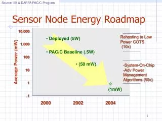
Source: ISI & DARPA PAC/C Program Sensor Node Energy Roadmap 10,000 1,000 100 10 1 .1 Rehosting to Low Power COTS (10x) • Deployed (5W) • PAC/C Baseline (.5W) Average Power (mW) • (50 mW) -System-On-Chip -Adv Power Management Algorithms (50x) (1mW) 2000 2002 2004
Source: ISI & DARPA PAC/C Program Communication/Computation Technology Projection Assume: 10kbit/sec. Radio, 10 m range. Large cost of communications relative to computation continues
Design Issues • Unattended Long Life • Communication is more energy-expensive than computation • 10E3 to 10E6 operations for the same energy to transmit one bit to 10-100 meters. • Self-organizing Ad hoc • Unpredictable and always changing. • Scalable • Scale to the size of networks • Requires distributed control
Sample Layered Architecture Source: Kurose’s slide User Queries, External Database In-network: Application processing, Data aggregation, Query processing Today’s lecture Data dissemination, storage, caching Congestion control Adaptive topology control, Routing MAC, Time, Location Phy: comm, sensing, actuation, SP
Impact of Data Aggregation in Wireless Sensor Networks Slides adapted from the slides from the authors B. Krishnamachari, D. Estrin, and S. Wicker
Aggregation in Sensor Networks • Redundant Data/events • Some services are amenable for in-network computations. • “The network is the sensor” • Communication can be more expensive than computation. • By performing “computation” on data en route to the sink, we can reduce the amount of data traffic in the network. • Increases energy efficiency as well as scalability • The bigger the network, the more computational resources.
source 2 source 1 source 2 Aggregates the data before routing it In this example average would aggregate to: <sum, count> source 1 & 2 Data Aggregation Temperature Reading (source 2) Temperature Reading (source 1) Give Me The Average Temperature? ( sink )
Transmission modesAC vs DC Source 1 Source 2 Source 1 Source 2 2 1 Data Aggregation 2 1 B A B A 1+2 1 2 Sink Sink • Address-Centric (AC) Routing • (no aggregation) b) Data-Centric (DC) Routing (in-network aggregation)
Theoretical Results on Aggregation • Let there be k sources located within a diameter X, each a distance di from the sink. Let NA, ND be the number of transmissions required with AC and optimal DC protocols respectively. 1. The following are bounds on ND: 2. Asymptotically, for fixed k, X, as d = min(di) is increased,
Theoretical results (DC) • ND Upper bound. • k – 1 sources 1 source nearest sink • Each X hop away: ( k – 1 )X + min(di) • ND Lower bound • if X = 1 or all sources are at one hop to the nearest source. • NA: >= k min(di)
Optimal Aggregation TreeSteiner Trees *A minimum-weight tree connecting a designated set of vertices, called terminals, in a weighted graph or points in a space. The tree may include non- terminals, which are called Steiner vertices or Steiner points 5 2 2 b d g b d g 3 1 3 1 1 4 1 5 2 1 e h e h 1 2 2 1 a c f a 3 2 *Definition taken from the NIST site. http://www.nist.gov/dads/HTML/steinertree.html 3
Aggregation Techniques • Center at Nearest Source (CNSDC): All sources send the information first to the source nearest to the sink, which acts as the aggregator. • Shortest Path Tree (SPTDC): Opportunistically merge the shortest paths from each source wherever they overlap. • Greedy Incremental Tree (GITDC): Start with path from sink to nearest source. Successively add next nearest source to the existing tree.
Aggregation Techniques Cluster Head Nearest source Shortest path Shortest paths SINK SINK a) Clustering based CNS b) Shortest Path Tree c) Greedy Incremental
Energy Costs in Event-Radius Model As R increases, the number of hops to the sink increases. CNS approaches the optimal when R is large.
Energy Costs in Event-Radius Model More saving with more sources
GIT does not achieve optimal Energy Costs in Random Sources Model
Aggregation Delay in Event-Radius Model • In AC protocols, there is no aggregation delay. Data can start arriving with a latency proportional to the distance of the nearest source to the sink. In DC protocols the worst case delay is proportional to the distance of the farthest source from the sink.
Aggregation Delay in Random Sources Model Although bigger in energy saving, it incurs more latency.
Conclusions • Data aggregation can result in significant energy savings for a wide range of operational scenarios • Although NP-hard in general, polynomial heuristics such as the opportunistic SPTDC and greedy GITDC are near-optimal in general and can provide optimal solutions in useful special cases. • The gains from aggregation are paid for with potentially higher delay.
Congestion Control in WirelessSensor Networks Adapted from the slides from: Kurose and Ross, Computer Networking, A top-down approach. Mitigating Congestion in Wireless Sensor Networks, B. Hull et al.
Congestion: informally: “too many sources sending too much data too fast for the network to handle” different from flow control! manifestations: lost packets (buffer overflow at routers) long delays (queueing in router buffers) a top-10 problem! Principles of Congestion Control
two senders, two receivers one router, infinite buffers no retransmission large delays when congested maximum achievable throughput lout lin : original data unlimited shared output link buffers Host A Host B Causes/costs of congestion scenario 1
one router, finite buffers sender retransmission of lost packet Causes/costs of congestion scenario 2 Host A lout lin : original data l'in : original data, plus retransmitted data Host B finite shared output link buffers
always: (goodput) “perfect” retransmission only when loss: retransmission of delayed (not lost) packet makes larger than perfect case for same l l l > = l l l R/2 in in in R/2 R/2 out out out R/3 lout lout lout R/4 R/2 R/2 R/2 lin lin lin a. b. c. Causes/costs of congestionscenario 2 “costs” of congestion: • more work (retrans) for given “goodput” • unneeded retransmissions: link carries multiple copies of pkt
four senders multihop paths timeout/retransmit l l in in Host A Host B Causes/costs of congestionscenario 3 Q:what happens as and increase ? lout lin : original data l'in : original data, plus retransmitted data finite shared output link buffers
Host A Host B Causes/costs of congestion scenario 3 lout Congestion Collapse Another “cost” of congestion: • when packet dropped, any “upstream transmission capacity used for that packet was wasted!
Goals of congestion control • Efficient use of network resources • Try to keep input rate as close to output rate while keeping network utilization high. • Fairness • Many flows competing for resources; flows need to share resources • No starvation. • Many fairness definitions • Equitable use is not necessarily fair.
Congestion is a problem in wireless networks • Difficult to provision bandwidth in wireless networks • Unpredictable, time-varying channel • A channel (i.e., air) shared by multiple neighboring nodes. • Network size, density variable • Diverse traffic patterns • But if unmanaged, congestion leads to congestion collapse.
Outline • Quantify the problem in a sensor network testbed • Examine techniques to detect and react to congestion • Evaluate the techniques • Individually and in concert • Explain which ones work and why
Investigating congestion • 55-node Mica2 sensor network • Multiple hops • Traffic pattern • All nodes route to one sink • B-MAC [Polastre], a CSMA MAC layer 16,076 sq. ft. 100 ft.
Why does channel quality degrade? • Wireless is a shared medium • Hidden terminal collisions • Many far-away transmissions corrupt packets Receiver Sender
Hop-by-hop flow control • Queue occupancy-based congestion detection • Each node has an output packet queue • Monitor instantaneous output queue occupancy • If queue occupancy exceeds α, indicate local congestion
0 1 Hop-by-hop congestion control • Hop-by-hop backpressure • Every packet header has a congestion bit • If locally congested, set congestion bit • Snoop downstream traffic of parent • Congestion-aware MAC • Priority to congested nodes Packet
Source rate limiting Count your parent’s number of sourcing descendents (N). Send one (per source) only after the parent sends N. Limit your sourced traffic rate, even if hop-by-hop flow control is not exerting backpressure Rate limiting
Related work • Hop-by-hop congestion control • Wan et al., SenSys 2003 • ATM, switched Ethernet networks • Rate limiting • Ee and Bajcsy, SenSys 2004 • Wan et al., SenSys 2003 • Woo and Culler, MobiCom 2001 • Prioritized MAC • Aad and Castelluccia, INFOCOM 2001
Evaluation setup • Periodic workload • Three link-level retransmits • All nodes route to one sink using ETX • Average five hops to sink • –10 dBM transmit power • 10 neighbors average 16,076 sq. ft. 100 ft.
2 packets from bottom node, no channel loss, 1 buffer drop, 1 received: η = 2/(1+2) = 2/3 1 packet, 3 transmits, 1 received: η = 1/3 Metric: network efficiency Interpretation: the fraction of transmissions that contribute to data delivery. • Penalizes • Dropped packets (buffer drops, channel losses) • Wasted retransmissions
Hop-by-hop CC conserves packets No congestion control Hop-by-hop CC
Metric: imbalance Interpretation: measure of how well a node can deliver received packets to its parent • ζ=1: deliver all received data • ζ ↑: more data not delivered i