Calibration of LAr and tile calorimeter cells at the EM scale

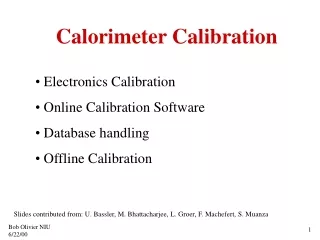
1. Calibration of LAr and tile calorimeter cells at the EM scale Manuella G. Vincter (Carleton University) • Many thanks to the organisers for asking me to give this tutorial • I have learned so much! • I’m a LAr/e- person but I’ll try to tell you what I’ve learned about the tile • My apologies if I don’t do the tile justice or misrepresent it. • I assume that you have a passing familiarity with our detector! • I won’t talk about the mechanics of our calorimeters • See our beautiful detector paper! • Menu for this presentation: • First 1/3 of the slides is the actual tutorial • I will try to spare you the nitty-gritty details • However, if you are up for some punishment, this little symbol invites you to look at the other 2/3 of the slides where many, many more details are given (in fine print). • I’ve received the help of many people to prepare this. Many thanks to them. Refs on the next page.

2. References (i.e. places from where I stole stuff) • Guillaume, Guillaume, Guillaume, Guillaume, Guillaume, Guillaume, Guillaume, Guillaume, Guillaume, Guillaume • Marco, Marco, Marco, Marco, Marco, Marco, Marco, Marco, Marco, Marco, Marco, Marco, Marco, Marco, Marco • M. Aharrouche et al Response Uniformity of the ATLAS liquid Argon EM calorimeter NIMA582 (2007) 429-455 • C. Gabaldon ATL-LARG-PUB-2008-001 • M. Aleksa et al., Combined TB: computation and validation of the elec calib constants for EM calo ATL-LARG-PUB-2006-003 • C. Collard et al., Prediction of signal amplitude and shape for the ATLAS electromagnetic calorimeter, ATL-LARG-2007-010 • J. Labbe, R. Ishmukhametov Crosstalk measurements in the EM calo during ATLAS final installation ATL-COM-LARG-2008-012 • LAr TDR & Calorimeter performance TDR • H. Brettel et al., Calibration of the ATLAS Hadronic Endcap Calorimeter. Conference proceeding of LECC workshop in Krakow • L Kurchaninov, Sept 2000 LAr week presentation+ CALOR 2000 • B. Dowler et al., Performance of the ATLAS hadronic endcap calorimeter in beamtests. NIMA482 (2002) 94 • J.P Archambault et al Energy calibration of the ATLAS Liquid argon Forward Calorimeter, JINST3 (2008) P02002 • Us et al., ATLASdetector paper • Design of the front-end analog electronics for the ATLAS tile calorimeter, K. Anderson et al., NIM A551 (2005) 469 • P. Adragna et al., Testbeam Studies of the Production modules of the ATLAS tile Calorimeter, Draft copy • K.J. Anderson et al., Performance and calib of the TileCal Fast Readout Using the CIS. ATL-TILECAL-INT-2008-002 • B. Salvachua et al., Online E & phase reco during commissioning phase of the ATLAS Tile Calo, ATL-COM-TILECAL-2008-004 • J. Poveda et al., Offline validation and performance of the TileCal Optimal Filtering reco algo, ATL-TILECAL-2009-001 • Richard Teuscher, Lukas Pribyl, Irene Vichou • L. Serin, V. Tisserand, Study of Pileup in the ATLAS EM calo, ATL-CAL-95-073 • W. Lampl et al., Digitization of LAr calorimeter for CSC simulations, ATL-LARG-PUB-2007-011 • G. Unal, Signal reconstruction in LAr, Jet Etmiss meeting, Feb 13/2008 • Us et al., CSC: Calibration and Performance of the Electromagnetic Calorimeter • F. Djama, Using Z to ee for Electromagnetic Calorimeter Calibration ATL-LARG-2004-008 • V. Gallo “Study of E/p with inclusive electrons from heavy flavours”, Mar 25/09 egamma meeting • F. Hubaut et al. Study of material in front of EM calo with high pT electrons, ATL-PHYS-INT-2008-026 • + other places I can’t quite remember…

3. ROD: online E reco Optimal Filtering LAr Front end L1A N samples Digitised ionisation scintillation Tile Front end Shaped signal L1A PMT signal N samples Digitised =GeV? Calorimeter overview E(GeV) Answers to all your secret questions… • Why do we turn the LAr pulse into that squiggly wave? • Why don’t we turn the tile pulse into a squiggly wave? • Why is it so hard to predict the LAr wave? • Why does tile have a zillion calibration systems? • What is that Optimal Filtering thingy? • And other details that you’ve always worried about… How to convert what the detector sees into an energy, in GeV, at the EM scale?

4. S2 S1,S3 EMEC drift time Mphys/Mcali EMEC Ion Cal  FCal Mphys/Mcali Barrel S2 S3 PS S1 LAr wave: before shaping I e/ penetrate calo: produce an EM cascade. Charged component ionises LAr in gaps, electrons induce triangular current signal, Iion(t). • Amplitude of signal: proportional to energy of particle in LAr • Length of signal: drift time of electrons in LAr gap • ~60115ns (FCal13) • ~450ns (HEC) • ~450ns (EMB), ~200600ns (EMEC) • LAr signal spans up to 24 bunch crossings! Looooooong! • Pileup? See later. To calibrate: inject known current to simulate LAr signal • Exponential calibration pulse Ical(t) mimics signal • difference in shape introduces Ereco bias: Mphys/Mcali • ~1.06-1.13 EMB, ~0.95-1.15 EMEC, ~1.020-1.025 HEC, 1 FCal • Corrected for in the energy reconstruction • Other bias also related to shape

5. Ion Shaped LAr wave: injection point, shaping, sampling Injection point of calibration pulse different for various detectors • FCal: at the baseplane of front-end electronics crate! • normalised physics pulse shapes come from test beam • HEC: injected right at the pad level, in front of cold preamps • Calibration and physics pulses fed through the same chain • EM: input to motherboard, point closest to signals from electrodes • Model of LAr wave needs to take this into account LAr wave is shaped • Bipolar, total area=0. Reason evident when we talk about pileup! • dynamical range of calo signals (MeV to TeV scale) requires 16 bits • analogue-to-digital converter (ADC) modules limited to 12 bits • shapers produce signals in 3 gains (low, medium, high) in ratio: 1, 9.3 and 93 • HEC: usually only in medium&low, PS: high&medium LAr wave is sampled at bunch-crossing frequency of 40MHz (25ns) • Upon L1A, up to 32 samples digitised (ADC), sent to ROD for E reco • in normal physics running: 5 samples • Cosmics: good to have as many samples as possible See for full details of the LAr readout.

6. Mphys/Mcali A Noise (1 sample)/(5 samples) gi = normalised pulse shape g’i = derivative of gi t EMEC LAr wave: shape prediction, optimal filtering Shape prediction: reconstruct E, need to know (normalised) pulse shape • Predict physics pulse gion(t) from calibration pulse gcal(t): • EM: gion(t)= gcal(t) x [Difference: shapes] x [Difference: injection point] • resistive component of inductance in calib board, decay of ion signal, drift time • cell capacitance (C) , inductive path ion signal (L), contact R cell&readout line • measurements or response to calib pulse: Response Transformation Method • Main systematic in Ereco :<0.5% (EMEC) determination o=1/√LC, EMB: precision of calib system: 0.23% • HEC pulse prediction tested with TB: residua <0.5% Energy reconstruction with Optimal Filtering (OF) • Usually 5 signal samples Si [ADC], 25ns apart (&pedestal, p) • Wish to reconstruct the amplitude A and time (phase)  a,b=OF coefficients • A: estimate E (aigi=1), no contributions from time jitter (aig’i=0) • ai, bi: minimise dispersion in A&A due to electronic noise&pileup • Get a quality factor on extraction of OFC: • out of time deposits, problems with pulse • Proof of noise reduction: apply OFC’s to pedestal sums • TB saw HEC: ~1.7, FCal: ~1.4, EMB~1.6, EMEC • For zero lumi & 5 samples, best reduction factor of ~2

7. i Electronic noise (MeV) Contributions non-uniformity: EMB <0.5% (~0.7% EMEC) LAr cell-level energy (EM scale) i=1 normally 5 Ramps (ADC to DAC) Signal (ADC) Peds (ADC) OFC TB: response to electrons +MC/geo to extrapolate 76.295V/Rinj Rinj= injection (EM) HEC: 0.017 A/DAC FCal1: 0.277 A/DAC FCal2: 0.269 A/DAC FCal3: 0.279 A/DAC EM: ~0.95-1.15 HEC:~1.020-1.025 FCal: 1 LAr calibration runs: Pedestal run (noise&autocorrelation) Ramp runs (gain of each cell) Delay runs (cell response to input current w/ programmable delay: gcal(t)) Note: inverse!

8. ETRec/ETTruth State of calibration with early data • Electronics calibration&TB: give us calibrated calo with a local constant term ~0.5-0.7% • If our MC correctly describes our detector material, then EM energy scale should look like: • This level of calib good enough for EM&jet physics with 2009-10 data • Check of E calibration with e from heavy flavours: bbeX (messy environment but plentiful) • look at peak of E/p (should be =1) • 1000 events/cell: E/p peak precision ~0.001 • 150pb-1: ~1000 “tight” e per layer-2 calo cell • Understand biases in ETRec/ETtruth and pTtruth/pTRec • compare bbeX with Zee and single ET • Next step is to look at E/p • Zee intercalibration: not for early running • Need lots of Z’s and must understand material Linearity Resolution Calibration hits method ||

9. A longitudinal shower variable A transverse shower variable Fraction in tails pTtrue/pTtrack and ETclus/pTtrack Material mapping • Energy calibration based on Monte Carlo • Likely that see deviations between MC and real data • Will need to verify detector description • ~3-12X0 before the EM calo, distributed in  • Unexpected material in detector will impact shower variables • Study with We CSC sample: impact of extra material on shower-shape variables • ~400pb-1 verify mapping to ~0.05Xo (stat only!) • Map conversion and brem vertices • Tails of E/p distributions due to early brem in the detector • map some aspects of the ID material, mainly pixels • Brem in SCT and TRT contribute little to tails • ~150pb-1 We, fraction in tails of ETReco/pTReco: pixel material could be tested at few % Xo

10. PMT signal Laser Clear fibre PMT Shaped signal CIS injects known current into readout. Shape similar to PMT pulse. WS Fibre Tile Cs holes Cesium source Laser system Charge Injection system Tile signal • Ionising particles crossing tiles induce UV scintillation light, converted to visible light by wavelength-shifting fibres. Readout out by PMT’s. • PMT signal ~18ns FWHM. • Shaped differential signals (50ns FWHM) in 2 gains (64:1) • System can accommodate full range of ~15MeV to 1.5TeV • Pulse is narrow compared to LAr wave (50ns vs 450ns)! • Digitiser samples pulse every 25ns with an ADC for each gain • After L1A, normally 7 samples (up to 16) sent to the ROD • Amplitude proportional to input charge and hence energy! • relate signal to input energy: calibration • Elements of the signal path • Scint tiles+WS fibres  PMT  electronics readout  ROD • Every aspect needs to be calibrated • See for full details of the tile readout

11. Pulse Charge injection system • CIS: calibrate front-end shaping and digitising • CIS and PMT signals use the same readout path • Inject calibrated charge in each channel via two capacitors (each gain) in steps over full range • From that extract calibration factors (H gain: 81.3ADC/pC, L gain: 1.29ADC/pC, both with RMS~1.5%) • Note: Signal produced similar to PMT but ~10% narrower & higher • Requires different references pulses for data and calibration • Total uncertainty on charge measurements on a single channel: 0.7% and from ADC resolution: 0.5 counts (solid lines) • Elec noise contributes for single channel measurements (dashed) • Systematic <1%, single channels measurements over most of range.

12. 3 cells Cs source and laser system • Cs calibration system • Measure quality of optical response of each cell, equalise signals by setting PMT HV, maintain stability of energy calibration • 1mm 137Cs source zooms through holes at edge of each of the 463k tiles and look at tile response • Different path: to a charge integrator in 3-in-1 card+ADC • PMT HV adjusted in iterative process to reach target value for response • Accuracy single tile response <2%, avg cell amplitude <0.3% • Short-term stability of system: ~0.5% • Laser system • monitor stability of PMT gains during physics&calib runs • pulses split close to the laser: small fixed fraction sent photodiodes for monitoring the relative pulse-to-pulse intensity. Balance sent to PMT’s through clear fibres • Test beam: global nonlinearity of PMT’s • <0.3%: 80–700 pC, 0.7%: 5-80 pC, 1.0%: 0.7-5 pC. X

13. D =∞ BC =0.35 A 200 cells 1.050pC/GeV A BC D Open: MC Closed: projective  TB  Cs hole Tile Tile: EM calibration constant • 1pC = ?GeV • Cell-level EM calibration constant, EMGeVpC, from TB&calib runs • TB: 20-180GeV electrons at ~0.35 • EM=1.0500.003 pC/GeV (stat) • Cell-to-cell response varies by 2.4% • But only checks row of cells closest to beam (A row) • Electron beam does not (much) penetrate to BC and D rows • Extend to other depths: TB e &  incident at =∞ • EM scale needs depth correction factors • PMT equalisation: assumes Cs source characterises response of scintillators to EM showers • Cs source always passes at edge of tile • Response at outer edge greater than at centre: 1%/cm • Larger tiles at larger radii • TB: Uniformity of response to  vs  • overall spread: RMS ~2.5% Full:  Open: e

14. OF2: Cosmics Tile: energy reconstruction Fit method: Optimal filtering (OF) method: • as described for LAr (OF1 method) • OF2 method: extract pedestal OFC as well • Shape derived for high and low gain channels in physics and calibration (CIS and laser) • Method used at ROD level • Only used fairly recently for offline • Mostly “Fit method” used offline (including TB) until recently • Results similar between fit method and OF (with iterations) • Same Ereco and noise

15. OF2: OF1: Tile cell-level energy (EM scale) Ecell = Cs xAOFC[ADC] [EMGeVpC]-1x [FpCADC]-1 x LAS x CIS: 82 ADC/pC (HG) 1.3 ADC/pC (LG)+ [Non-linear corr] (RMS~1.5%) Laser: 1 + [non- linear corr] (RMS<0.5% over days) Cs: 1 + [corrs for D cells & special cells] [TB(e-): 1.050pC/GeV/ [R corr] (RMS~2.4%) Equalise PMT response (set HV) TB uniformity: Ecell ~2.5% (electrons) ~1.5% (hadrons) independent of  Cs: RMS drift after 4 months <1% (with no corrs) TB(@90o): Correct for radial dependence response@A/@BC or D

16. 10GeV LAr signal (interesting event) Electronics+pileup noise/cell (2x1033) Pileup Electronic noise (MeV) LAr Tile If not shaped: x 18-23 Shaped signal PMT signal Fast facts about pileup • Number of inelastic collisions per bunch crossing <N> = inel xL x Dt / eoccupancybunch • <N> = ~70-80 mb x 1034 cm-2 s-1 x 25 ns / 0.8 = 20-25 • ~23 simultaneous collisions/BC at 1034 cm-2 s-1 • ~2.3 at 1033 cm-2 s-1 • For our detector, at 1034 cm-2 s-1 every bunch crossing: • ~900 charged tracks through inner detector! • ~1400 GeV of ET (~3000 particles) in calos • <pT> charged (neutral): ~0.5-0.6 (0.3)GeV • Tile pulse quite narrow: PMT signal <1BC, shaped~4BC • LAr wave wide! 18-24 BC (FCal: 3-5 BC) • Pileup could contribute significantly to the signal

17. Zero lumi 1033 ~0.8x1034 1MB in one cell (MeV EM scale) Peaking time: 5%- 100% -3/2 1/2 Pileup and the LAr wave • LAr wave shaped to compensate such that area=0 • positive lobe, with negative lobe: provides cancelation • Note: due to shape of wave & ET spectrum, area=0&avg=0, but most probable value of energy is not! • For one sample: • 2E = RMS of E deposit/MB, N= #collisions/BC, NB=#BC, ~2 • depends on LAr wave, g! • N~222pileup =442E (@1034); N~22pileup =42E (@1033) • Note: pileup noise not gaussian. Noise correlated between samples • Contributes to the noise autocorrelation function • Shaping time of LAr wave chosen to minimise total noise but… • Depends on lumi and  • choose peaking time of LAr wave of ~40ns (but OFC can be optimised offline by software) • Noise grows: (x)0.75(EM,HEC)-0.85(FCal) • E offset scales as NcellsEoffsetcell

18. Predicted noise after OFC (5 samples) for 2 EM cells vs lumi Pileup e-noise Pileup e-noise =0.6 =3.0 Impact of pileup on OFC’s • LAr OFC calc requires physics pulse shape (lumi indep), total time autocorrelation function (lumi dependent!) • LAr online OFC’s will only be updated in between fills • Has impact on the noise reduction during a fill: • 5% if optimise @1034 but fill varies 0.5-1.5x1034 • Tile pulse narrower then LAr pulse • pileup will have less of an impact • Tile pulse is unipolar • No cancellation like for LAr • Baseline calculated for every event! • Pileup contributes to occupancy and deposits energy • Fluctuations contribute to noise term of resolution, especially for hadronic jets which have lots of cells • Cell A12: first layer of Tile. e.g. 1034cm-2s-1 • M=mean occupancy: prob that signal >1MeV observed in cell = 22% • E=deposited E per cell per BC=27MeV • OFC: sizeable impact in A layer, dominant contribution is elec noise • Impact on amplitude at 4.6 colls/BC in the absence of elec noise Tile

19. Cluster energy (MeV) EM IW: ~3, after OFC, 1034 … Bunch structure Cluster energy (MeV) 3x: 25ns75ns ~21 (missing terms in sum) Impact of beam structure on LAr energy • Holes in the beam structure! Impacts compensation provided by undershoot of LAr wave • Not too bad for barrel: 40MeV in ET, negligible increase in noise • Endcaps ~3: 500MeV shift in cluster E, 50MeV in ET and 10% increase in noise • Shift measured in physics randoms, using non-empty bunches, correct average offset • Could be corrected offline vs bunch number but implementation will be tricky! • Previous studies shown to not be an issue for the trigger • Going from 25ns to 75ns bunch crossing times: • For equivalent lumi as at 25ns: pileup gets worse! • Get more irreducible pileup (can’t be minimised as well by OFC) • e.g. EM IW layer 1: increase in pileup noise of 40% • May have some visible energy shift • Extreme case 1BC per 100’s of ns: shift ~N x EMB • But won’t this phase be at low lumi anyway? Don't worry! Be happy!

20. That’s all folks! Thanks for attending this tutorial. See extra slides for more info…

21. Menu of extra goodies… LAr: energy reconstruction Optimal filtering coefficients computation Tile: energy reconstruction OF timing: LAr and Tile LAr: calib constants (EM scale) Tile: calib constants (EM scale) I Tile: calib constants (EM scale) II Collisions per bunch crossing Pileup and the LAr wave Impact of pileup on LAr OFC Impact of pileup on Tile OFC Calorimeter granularity LAr readout, in a nut shell Tile readout, in a nut shell LAr: relating physics&calibration pulses Differences: HEC and FCal Tile: relating physics&calibration pulses LAr: pedestals&autocorrelations LAr: ramps and delays EM Crosstalk Tile: charge injection and laser Tile: Cs source and MB current e/ cluster energy reconstruction EM calo calibration with Zee

22. Calorimeter granularity EM calo Tile calo

23. LAr readout, in a nut shell The readout signal: sum of signals measured in electrodes • Summing boards: analogue sum at both ends of electrodes • Motherboards: on top of the summing boards, readout sum, send signals out the cryostat, distribute calibration signal The calibration pulse: • EM: injected at the analogue input to the mother-board • HEC: injected in front of the cold preamps • FCal: injected at base-plane of the front-end crates, where the signals are split into two parts • One into the front-end boards: calibrate the electronics • One through the cold electronics chain, reflects off the electrodes, is observed as a delayed pulse: examine problems related to the FCal and its cold electronics Front-end crate contains boards for: • Calibration: injects known pulses through resistors • Front-end readout boards (FEB) • Tower builder/driver: form trigger-tower signals and transmit analogue signals to the L1 trigger processor • Controller: receive/distribute the 40MHz clock, the L1 trigger accept signal, configure/control FEB • Transmit detector “stress” info: LAr purity, temp etc… Front-end boards: • Preamps: amplify raw calorimeter signals • Shaper: applies bipolar analogue filter to optimise signal-to-noise ratio: • A differentiation step removes long tail from detector response • Two integrations limit bandwidth to reduce noise • Note: Energy dynamical range requires 16 bits but ADC modules limited to 12 bits • shapers produce 3 signals amplified in 3 gains: low, medium and high (1:9.3:93) Switched-capacitor array (SCA): • Signal sampled LHC bunch-crossing frequency of 40MHz • Stores signals during the L1 trigger latency • L1 accept events: typically five samples per channel in one of the three gain scales are read out Signal transmitted by optical transmitter to the ROD ROD (ReadoutDriver) • receive and digitally process/format data from FE electronics • perform data-integrity checks & high-level monitoring • Perform event averaging for calibration runs • ROD module: motherboard has up to 4 processing units (PU) cards. Each PU has 2 Digital Signal Processing (DSP) chips. • DSP: applies Optimal Filtering to signals to provide signal in GeV, timing for each cell, and quality factor.

24. Front-end electronics located in 3-m-long drawers at outer radius of the calo. Contain: PMT’s, HV distribution system, and front-end analog (3-in-1 cards) and digital electronics Signal path: Shape the 18ns FWHM PMT signal produce two linear outputs with relative gain of 64 (high and low gain) for 16-bit dynamic range Measure E deposition of 15MeV to 1.5TeV/cell Output pulse: quasi-Gaussian ~50ns FWHM and peak ~70 ns after the input pulse digitiser system samples the shaped signals every 25ns with two 10 bit ADCs (low-gain&high-gain), stores up to 16 samples in pipeline, waiting L1A. Normal data-taking mode: 7 samples are kept digitised data transferred by optical link to ROD’s RMS variation in output amplitude from board to board expected to be 0.2% Sensitivity of output pulse amplitude to changes in the input shape: varying fall time of input pulse by 5 ns -2.8% and +2.0% change in magnitude of the peak sample (for sampling synchronized to the timing of the input pulse). 1.5 ns shift in the time of output peak Integrator: low-pass DC amplifier integrate PMT current induced by Cs source as it traverses holes through the scintillating tiles measure PMT current induced by minimum bias events During Cs calibration: a resolution >1% is achieved, non-linearity of system <0.3%. Charge injection system (CIS): Inject signals similar to PMT signals (but FWHM 10% narrower and amplitude 10% higher, difference can be measured with physics events) and of precisely known amplitude over the full dynamic range 100 pF capacitor of 1% tolerance charged with high-precision voltage source & discharged into input electronics. allows an injected charge of over 800 pC in steps of 0.8 pC (for low-gain) 5.1 pF capacitor of 2% tolerance is used signals up to 40 pC in steps of 40 fC (high-gain) uncertainty in the measured PMT charge arising from the electronic readout system is less that 0.7% Trigger: Provide differential signals for trigger adder cards perform the analog sums of the signals within the trigger towers of every module Tile readout, in a nut shell

25. Diff: injection pt phys&cali Diff: phys&cali shapes: fs, c, TD LAr: relating physics&calibration pulses I • EM cells modelled as resonant rLC circuit • C = cell capacitance • L=inductive path of the ion signal • r= contact r betw cell & readout line • Output physics pulse gion(t) predicted from calib pulse gcal(t) by factorising the readout chain transfer function via time-domain convolutions • When e/ hit the calo they produce an EM cascade. Charged component ionises the LAr in the gaps, inducing a triangular current signal, Iion(t). • TD = drift time • Exponential calibration pulse Ical(t)) mimics this ionisation pulse. • fs=resistive component of inductance in calib board • c= decay of ion signal • All parameters either from measurement or RTM method (or both!) • fs~0.08, c~400ns (lab measurement or RTM method) • TD~gb+1/Ub, b~0.4, U=applied V, g=gap thickness or from TB with 10% precision • Resonant o with network analyser: o=1/√LC and r=rc (r from pulse amplitude at resonance, C measured after module stacking or from RTM) • Sources of systematics: RTM-measured: • c=-7%, fs=+15% • r~ factor 2-3 (3-5) barrel (endcaps) • r0 in S1&S3 endcaps • o ~10-15% at high  (~1% in barrel) • Up to ~0.5% sys in E reco in endcap • To be absorbed with intercalib from Zee? • Expect <0.2% uncertainty

26. Differences: HEC and FCal HEC • Influence of the calibration accuracy on the jet energy resolution: imperfections of the electronics are propagated only to the constant term of the jet energy resolution formula. Calibration system accuracy must be better than 1%. • HEC calibration signal injected in front of cold preamps • ionisation current fed through same path as calib • Prediction of particle response from measured calib. • a relationship between normalised calibration pulse TC(t) and predicted signal pulse Tp(t): numerical reconstruction method • Electronic response Ha(s) factorised out • Tested with 100GeV electrons: residua <0.5% FCal • Calibration pulse injected at base-plane of the front-end crates, not at the detector level • Master pulse shapes obtained from test beam data • Pulse shapes reconstructed from test beam data by starting with a prediction from SPICE model of electronics chain and performing an iterative fit • Electronics noise from TB and fed back into SPICE • Pulse shape differs per module due to difference in drift time due to LAr gap, but shape is stable per channel within a module • One normalised pulse shape used per module

27. Mphys/Mcali Barrel S2 S3 S2 PS S1 S1,S3 LAr: relating physics&calibration pulses II • Difference between shapes of the physics and calibration pulses introduces a bias in energy reco • Use ratio of the maximum amplitude of the two pulses: Mphys/Mcali • decreasing behaviour with  reflects cell inductance and drift time variations • Note: prediction of this bias on the signal reconstruction method can’t rigorously verified with cosmics: absolute muon energy scale only known at ~5% • uncertainties will be absorbed in the inter-calibration coefficients from Zee decay. Note1: HEC • calibration pulses injected in front of cold preamps • Each cell injected with up to 4 calibration pulses (these large cell size are readout with up to 4 preamps) • Will get up to 4 calibration objects for from cell which will have to be averaged. • Mphys/Mcali =1.020-1.025 (medium gain) Note2: FCal • Does not predict ionisation pulses from calibration • Uses TB results as primary input and SPICE MC (incredibly uniform within a module!) • Mphys/Mcali =1

28. 2008 cosmics noise Pulse Derivative Tile: relating physics&calibration pulses I Pulse shape (and its derivative): • Needed for energy reconstruction (fit and optimal filtering methods) Physics signal: • PMT 18ns: FWHM PMT signal • Output pulse: quasi-Gaussian ~50ns FWHM • Electronic noise: • Typical pedestals: ~30-60ADC • Typical noise: ~1.2ADC (high gain), 0.6ADC (low gain) • So far obtained from TB and commissioning (both asynchronous) Calibration pulse: • for different types of runs, in both gains • Laser • CIS • Is different from physics pulse

29. Tile: relating physics&calibration pulses II Calibration pulse: obtained from CIS runs • Signal produced by calibration capacitor similar in shape to the signal produced by PMT but has a full width at half maximum (FWHM) about 10% narrower and an amplitude 10% higher than a PMT signal of the same charge. • CIS system injects a small bipolar transient signal into the passive shaper: “leakage pulse” • low gain peak amplitudes: 1.2 counts (0.9 pC) and 0.7 counts (0.5 pC) for the 100 and 5.2 pF capacitors • high gain the corresponding amplitudes are 65 counts (0.79 pC) and 25 counts (0.31 pC) • present only in CIS data and not in physics data • Measured and subtracted to get reference pulse • Low gain non-linearity correction (~2%): both calib and real data • Total uncertainty on charge measurements on a single channel is 0.7% and from ADC resolution (0.5 counts): solid lines • Electronic noise contributes for single channel measurements: total is dashed lines. • Systematic uncertainty <1% for single channels measurements over most of the range. • Expected systematic uncertainty on mean response for test beam measurements with electrons and pions (at EM scale) as a function of the total measured charge. • Systematic uncertainty expected to be smaller for jets: more channels used in a measurement. Leakage pulse

30. Typical EMB autocorrelation values (TB) Typical EMB pedestal values (TB) 2 of pedestal Commissioning of the A side LAr calorimeters (high gain) Front back mid Noise (ADC) PS Front back mid Pedestals (ADC) Noise (ADC) EMBA pedestals Sample number EMBA noise EMECA (STD) noise Typical EMB normalised autocorrelation values HEC normally only in medlium&low gain IWA noise HECA noise all layers FCalA noise 1 2 3 Noise (ADC) Noise (ADC) Noise (ADC) S1 S2 Sample number LAr: pedestals&autocorrelations • Dedicated runs without beam or injected charge measuring the pedestal and autocorrelation matrix needed for the energy reconstruction. • Alternatively during physics runs, random triggers can be used to obtain the same information. • Pedestals: The mean (pedestal) and RMS (noise) is computed for each cell and gain by averaging over a given number of periodic triggers and over the number of samples. • Autocorrelation: Vij=<SiSj> where Si is the pedestal subtracted (ADC counts) in sample i, mean value over the total number of events (may be normalised by ij)

31. LAr: ramps and delays Ramps • Each cell pulsed N times with a set of given input currents (DAC values) a time delay =0 between the calib pulser and DAC, for each gain • Get ADC value over the N triggers each sample • Compute mean&RMS over the N triggers for each sample • Get averaged calibration wave for each DAC value • Get ADCpeak for each wave and plot vs DAC value • Linear interpolation to get the ADCpeak to DAC ramp coefficients: DAC = a + bADCpeak • Note: saturation plateau for ADCpeak corresponding to the maximum 12-bits ADC value (4096) minus the pedestal value (around 1000)≈3000 Delays • Each cell pulsed N times with a given input current (DAC value) at a given time delay between the calib pulser and DAC, for each gain • Get ADC value over the N triggers each sample • Compute mean&RMS over the N triggers for each sample • Delay is sequentially increased in steps (e.g. 1ns) until the sampling period is covered • Get averaged profile of the response of the cell to the input DAC • Pedestal subtracted to restore the proper baseline. Commissioning of the A side LAr calorimeters EMBA middle (high gain) EMBA middle (high gain) FCal1A (high gain) HECA (medium gain)

32. Middle-back Back-back Middle-middle EM Crosstalk A B • Crosstalk: signal leakage from a cell with a signal to other cells • modifies the position and the value of the signal channel peak • Can be measured peak-peak or under-peak • Corrected by adding contributions from neighbouring channels • Capacitive crosstalk: front layer • On the electrodes. Main source of cross-talk. • Signal from cell shared to neighbours and next-to-nearest neighbours • detector/crosstalk capacitance: Cd/Cx • Dispersion in  ~10% (peak-peak) • Resistive crosstalk: middle and front layers • HV supplied to front by resistors physically connected to middle cells • Difference for electrodes A and B • 1/ resistance for parallel-connected resistors located in front of the pulsed middle cell • Long distance: in front cell when signal sent to middle cell not connected to front cell • Dispersion in  ~15% (peak-peak) • Inductive crosstalk: middle and back layers • mutual inductance between the cells and from the ground return • look at  neighbour inside samplings or cells in front of pulsed one

33. Charge injection (CIS) calibration calibrate front-end shaping and digitising circuits to 1% Fast input pulses from a PMT or from the CIS use same readout chain. Inject calibrated charge into each channel via 2 capacitors 100 pF with 1% tolerance (low gain) 5.1 pF with 2% tolerance (high gain) signal produced similar to the PMT signal but FWHM ~10% narrower & amplitude ~10% higher Output Q the same for 2 sources of same Q: <1% Dedicated CIS runs: charge injected in steps over full range for both gains High gain: 81.3counts/pC, low gain: 1.29counts/pC, both RMS~1.5% TB: departure from linearity at low charge/gain ≤2 ADC count Can be corrected for with calibration TB: channel-to-channel gain: RMS variation of 1.5% 4-month 2004 TB, corrected gains stable: RMS <0.2% variations in gains: ADC & PMT anode capacitances After calibration: channel-to-channel sys error estimated to be ~0.7% + 0.5 counts uncertainty on ADC resolution. Laser system monitor stability of PMT gains to <1%, during physics and in calibration runs can also measure absolute gain of each PMT Frequency-doubled Nd :YVO4 laser, produces 532nm, 10ns pulses, synchronized to 40MHz clock pulses split close to the laser: small fixed fraction sent photodiodes for monitoring the relative pulse-to-pulse intensity. Balance sent to PMT’s through clear fibres TB: dispersion of relative gains of 40 PMT’s during 32 runs over 3 days: ~0.5% TB: Global nonlinearity of PMT’s: <0.3% in 80–700 pC, 0.7% in 5-80 pC, 1.0% in 0.7-5 pC. Response to CIS pulses 2pC (high gain) 560pC (low gain) Tile: charge injection&laser

34. Cs source scans enables the setting of HV to equalise response and inter-calibration of each channel to maintain stability of energy calibration to 0.5% dedicated runs, 137Cs–source traversing all 463k tiles 1-mm-long source, passes through water-filled holes/tubes at normal incidence in every tile and absorber plate Sees tile but uses diff path to a charge integrator in the 3-in-1 card + ADC Each PMT HV adjusted in an iterative process to reach target value for response Accuracy of single tile response <2% and average cell amplitude <0.3% short-term stability of system: 0.2% (0.5%, if water flushed and measurement repeated) characterises level of precision for monitoring the long-term cell response Tracking over 4 months of TB: RMS = 0.9% Minimum bias current Same charge integrator used to measure PMT current during Cs run can be used to monitor MB current during a physics run MB current produce occupancies in tile cells, but is ~constant over milliseconds Tile: Cs source and MB current 3 cells Typical cell

35. ai bi i=1 to 5 samples Si = signal (ADC) p = pedestal (ADC) gi = normalised pulse shape g’i = derivative of gi ai,bi= OF weights EMB A Noise (1 sample)/(5 samples) t LAr: energy reconstruction Optimal Filtering (OF) method implemented in all calorimeter ROD’s and used offline. NOTE: also used for Tile! • calculates amplitude A, timing  and simplified 2 for shaped & digitised signal from each cell: weighted sum over samples • OF coefficients ai, bi obtained by minimising dispersion in A and A due to noise (electronics and pile-up) • OF coefficients ai and bi computed for 50 phases&each gain • Takes into account noise-correlations between samples: Rij • A should estimate energy (ai gi=1) with no contribution from time jitter (aig’i=0) NB: FCal master waves used for OFC computation obtained from TB, not from calibration runs. Proof of noise reduction: apply OFC’s to pedestal sums for increasing number of samples • HEC: ~1.7, FCal: ~1.4, EMB, EMEC • Now you know why for cosmics we like to take so many samples!

36. Optimal filtering coefficients computation Choose coefficients for the expressions: such to minimize and with the constraints:  ,  , noise autocorrelation function

37. Fit Hatched: FF FWHM =50ns (phys) =45ns (calib) OFC weights Pedestal Phase Amplitude Cosmics Tile: energy reconstruction Flat filter (FF): • N digitised samples divided into a pedestal window (ped=average over window) and a signal window (signal=largest sum of successive samples, typically 5) • TB: Introduces a positive bias: channels without signal have an average amplitude ~10 MeV and RMS of~50 MeV Fit method: • Used mostly frequently until recently. Most recent offline running (including TB) uses this method • 2 minimisation for each channel fit to function f(t)=Ag(t-)+c to determine A=amplitude,  =phase (fixed during normal running), and c=pedestal given a normalised pulse shape g. • Pulse shape derived for high and low gain channels in physics and calibration (CIS and laser) • TB: introduces a positive bias of ~0.2MeV, with gaussian spread of noise 2x better than FF • TB: 11% difference in pC/GeV factor between FF and fit, but no impact on calo performance when taken into account • calibration constants agree at 1% level Optimal filtering (OF) method: • as described for LAr (OF1) • OF2: extract pedestal OFC as well • Used fairly recently for offline • Method used at ROD level • ~2x noise reduction compared to FF • ~results between fit and OF (with iterations) • Same E reco and noise • Without iterations, OF method narrower

38. Tile: TB FCal: TB EM: toy MC OF timing: LAr and Tile • For TB and cosmics, signals arrive asynchronously from the trigger clock • OF must be calculated through an iterative process • OF coefficients determined for different phase delays, usually in steps of 1ns • For LHC running, signals will arrive synchronously with LHC BC clock, to some level (few ns?) • Wrong timing will results in a degradation of the reconstructed energy. • Tile: fractional difference between reconstructed amplitude for fit and OF methods vs OF time • OF Amplitude ~0.5% low for timing 2ns off • LAr: • EM fractional error on OF Amplitude ~0.5% low for timing 5ns off • FCal: <0.5% low for timing 5ns off • For real running, these kinds of effects should be quickly determined and corrected.

39. i LAr: calib constants (EM scale) i=1 normally 5 Cell-level energy (EM scale) Ramps (ADC to DAC) OFC Signal (ADC) Peds (ADC) 76.295V Rinj Rinj= injection resistor on motherboard (EM) HEC: 0.017 A/DAC FCal1: 0.277 A/DAC FCal2: 0.269 A/DAC FCal3: 0.279 A/DAC EM: ~0.95-1.15 HEC: ~1.020-1.025 FCal: 1 Electronic noise (MeV) Note: inverse!

40. 3 barrel modules Open: MC Closed: projective  Tile: calib constants (EM scale) I • Cell-level EM calibration constant: Ce, determined from TB and calibration runs • TB: 20-180GeV electrons at ~0.35 (20o) only checks A-row cells • EM=1.0500.003 pC/GeV (stat) • Cell-to-cell response varies by 2.4%, due to differences in light yield and non-uniformity of light collection within tiles, tile-to-fibre optical coupling, conversion efficiencies&transmission in fibres, PMT variation of response • Cs scan: individual tile response over a whole module: RMS~5% • Readout electronics: systematics due to charge injection calibration and ADC’s <0.7% (E>20GeV). Due to charge integrator: <0.5% • TB: extend to other tile depths: electrons and muons incident at =∞ (90o) • Muons: apply EM=1.050 and e/ response=0.91. Signals: energy/ path-length • EM scale needs depth correction factors • equalisation of PMT signals based on response of every tile-row to Cs source signal and on assumption it characterises the response of scintillators to EM showers. Near outer edges (where the Cs signals produced) response is greater than at the centre, by about 1%/cm radial distance from the center. Larger tiles at greater radii • Normalised to 1 in A row (to preserve electron results), inverse ratio of the mean muon response in the other tile-rows to that in the A-cell tile-rows • TB: Uniformity of response to muons vs  • Projective muons in centre of each tower. Span −1.45<<1.35 in steps of 0.1 • overall spread: RMS ~2.5% • TB: EM linearity with electrons at ~0.35 (20o) • Small ~0.5% non-linearity due to iron front plate • 3% fluctuations, mostly due to tile-to-tile differences • difficult to decouple from reproducibility of aim of e-beam • TB: • A=28% GeV-1/2, b=2.8% • Note: in real running, Tile won’t “see” electrons • All absorbed in LAr calorimeter!

41. OF2: OF1: Tile: calib constants (EM scale) II Ecell = Cs xAOFC[ADC] [EMGeVpC]-1x [FpCADC]-1 x LAS x CIS: 82 ADC/pC (HG) 1.3 ADC/pC (LG)+ [Non-linear corr] (RMS~1.5%) Laser: 1 + [non- linear corr] (RMS<0.5% over days) Cs: 1 + [corrs for D cells & special cells] [TB(e-): 1.050pC/GeV]/ [Radial corr] (RMS~2.4%) Equalise PMT response (set HV) Cs: RMS drift after 4 months <1% (with no corrections) TB(@90o): Correct for radial dependence response@A/@BC or D

42. no pile-up added LHC design luminosity pile-up added Et ~ 81 GeV Charged particle multiplicity and energy in pp inelastic events at s = 14 TeV Et ~ 58 GeV <pT> ~ 600 MeV Collisions per bunch crossing • Impact of many minimum bias events in physics collisions: pileup • Extract number of inelastic collisions per bunch crossing <N> = inel xL x Dt / eoccupancybunch • LHC: <N> = ~70-80 mb x 1034 cm-2 s-1 x 25 ns / 0.8 = 20-25 • On average, ~23 simultaneous collisions per BC at 1034(~2 at 1033) • Physics is approximately constant as a function of  for fixed pT • Charged particle multiplicity: • dncharged/d 7.5 per  = 1, mostly ± with <pT>  0.6 GeV • dnneutral/d 7.5 per  = 1, mostly  from 0 with <pT>0.3GeV, • Most the energy from a p-p never makes it into the detector! • Detector coverage –2.5 << 2.5 (=9.4o) for tracks, –5 << 5 (=0.8o) for calo: • ~900 charged tracks every 25 ns through inner tracking • ~1400 GeV of Et (~3000 particles) in calorimeters every 25 ns • ~300000 GeV down the beam-pipe • Minimising the impact of pile-up on the detector performance: • precise&fast detector response minimises pile up in time • highly granular detector minimises pile up in space (numbers vary with models)

43. LAr signal (interesting event) Pileup 1MB in one cell (MeV EM scale) Peaking time: 5%- 100% -3/2 1/2 Pileup and the LAr wave • Typical LAr signal: triangular shape, with drift-time ~450-600ns, spans ~18-24 BC • Note: FCal shorter (50-100ns), Tile requires no shaping: FWHM~45ns • Each interesting signal would have sitting on top all the MB events in that cell • LAr wave shaped to compensate such that area=0: positive lobe and negative lobe • Note: due to shape of wave and Et spectrum, area=0, but most probable value is not! One sample: • 2E = RMS of E deposit/MB, N= #collisions/BC, NB=#BC, ~2 (depends on LAr wave!) • N~22  2pileup =44 2E (1034); N~2  2pileup =4 2E (1033) • Shaping time of LAr wave chosen to minimise total noise but… • Different for different luminosities •  dependent • chose peaking time ~40ns • Total noise grows as (x)0.75(EM,HEC)-0.85(FCal) and E offset scales and NcellsEoffsetcell Zero lumi 1033 ~0.8x1034 Electronics+pileup noise/cell 2x1033

44. 1.05 Noise using OFC@1034/Noise with optimised OFC 1.00 Lumi/1034 Impact of pileup on LAr OFC Predicted noise after OFC (5 samples) for 2 EM cells vs lumi • OFC calculation requires physics pulse shape (lumi independent), total time autocorrelation function (now lumi dependent!). Summation done over all relevant bunch crossings. • Need to include Rij if you want to effectively reduce impact of noise with OFC • Rij can be measured from random events during physics • OFC’s will only be updated in between fills • Has some impact on the noise reduction during a fill

45. High gain, real data A layer: electronic noise + 4.6 MB pileup Impact of pileup on Tile OFC • Tile pulse narrower then LAr pulse • pileup will have less of an impact • Tile pulse is unipolar • No cancellation like for LAr • Pileup will contribute to occupancy of cells and deposit a small amount of energy • Fluctuations contribute to noise term of calo resolution, especially for hadronic jets which have lots of cells • Cell A12: first layer of Tile. e.g. 1034 • M=mean occupancy: probability that a signal >1MeV is observed in cell ~22% • E=deposited E per cell per BC=27MeV • OF reconstruction requires autocorrelation matrix, rk • Consider only high gain where impact is biggest • Impact on OFC (4th sample) using unitary autcorr matrix to • Use on electronic noise only for autocorr • Use MB (4.6 collisions/BC) for autocorr • Sizeable impact in A layer only, but dominant contribution is still electronic noise • Impact on amplitude at 4.6 collisions/BC in the absence of electronic noise • Note the log scale! • Can be cleaned up with quality factor cut a4 ~0.8 at =0

46. Barrel e: 3×7 cells (S2); (un)converted : (3x5) 3×7 cells Endcap e/: 5×5 cells Cluster energy reconstruction electronics calibration at the cell level cell energy summed cluster position corrections (S-shape correction) sum cluster E in each layer: calibration hits method Ecal: energy deposited in EM calo Efront: energy deposited in PS and material in front of calo Eback: longitudinal leakage energy Reconstructed calo energy: Ecal: Ecl: cluster energy deposited in each layer X: shower depth (longitudinal barycentre) : cluster barycentre, corrected for S-shape Ccal(X,) energy calibration factor Ratio: true (absorbers+LAr) E to reco cluster Ecl fout=fraction of E deposited outside cluster Energy in front of the calo: Efront E lost in front of calo + PS and S1: 2nd order poly in EPS 1.8 <||<3.2, 2nd order poly in X Longitudinal leakage: Eback as a fraction of the energy reconstructed in the calorimeter Ccal vs X fout vs X Efront vs X Efront vs EPS Eback vs X ||=0.3 Eback vs X ||=1.65 /E vs || Sampling term vs || e/ cluster energy reconstruction: calibration hits method Non-linearity: <0.5% over full || range

47. EM calo calibration with Zee • Electronics calibration&TB give us calibrated calo with constant term ~0.5-0.7% but • perhaps only true in patches of x (local): need to intercalibrate to all regions • tell you little about the detector-related non-uniformities which can impact global energy calibration • Possible sources: • 2-12X0 of material before the EM calorimeter, non-uniformly distributed in  • Liquid argon temperature impact on EM signal: -2%/K • Temperature probes good to 10mK • Temperature of electronics (cooling water): • T=1oC  0.5‰ change in ramps&delays • HV fluctuations? • Not clear this method can give input to such short time scale issues! • Idea: use Z mass to intercalibrate all regions: global energy scale to ~0.1-0.2% • Parametrise long-range non-uniformities with Ereco=Etrue(1+i) • Can inject biases  as gaussian with mean and width • look at effect on invariant mass of electrons in two regions i,j • Fit to Mtrue by minimising the loglikelihood of the pdf, extract ,,M • Has been shown that introducing a fixed bias can be recovered • Used CSC production with distorted material • Provides an intrinsic bias to the data which can be measured • Conclusions from CSC note: • ~200 pb-1 of reconstructed Z → eeevents with an initial width of bias of 2% • long-range constant term ≤0.5% • overall constant term ~ 0.7% • Bias on the absolute energy small: ~0.2% • (Optimistially!) comparable to what we get with electronic and TB calibration • But, to look at such (time varying?) non-uniformities • Need a lot of Z’s statistics in a short period of time! • Need to understand material mapping. • This kind of study is for later data Bias in ideal and distorted geometries