Download

1 / 32
380 likes | 642 Vues
Review of Flood Routing. Philip B. Bedient Rice University. Lake Travis and Mansfield Dam. Lake Travis. Mansfield Dam, built in 1937. Lake Travis. Brays Bayou High Flow. 6 to 7 inches of Rainfall. T.S. Allison June 2001. Houston. Galveston Bay.

E N D
Review of Flood Routing Philip B. Bedient Rice University
Lake Travis and Mansfield Dam Lake Travis
Mansfield Dam, built in 1937 Lake Travis
Brays Bayou High Flow 6 to 7 inches of Rainfall
T.S. Allison June 2001
Houston Galveston Bay Hurricane Rita Landed on Sabine, TX On Sep 24, 2006
Detention Ponds • These ponds store and treat urban runoff and also provide flood control for the overall development. • Ponds constructed as amenities for the golf course and other community centers that were built up around them.
Reservoir Routing • Reservoir acts to store water and release through control structure later. • Inflow hydrograph • Outflow hydrograph • S - Q Relationship • Outflow peaks are reduced • Outflow timing is delayed Max Storage
Inflow and Outflow I1 + I2 – Q1 + Q2 S2 – S1 = 2 2 Dt
Inflow & Outflow Day 3 = change in storage / time Re Repeat for each day in progression
Determining Storage • Evaluate surface area at several different depths • Use available topographic maps or GIS based DEM sources (digital elevation map) • Outflow Q can be computed as function of depth for either pipes, orifices, or weirs or combinations
Typical Storage -Outflow • Plot of Storage in acre-ft vs. Outflow in cfs • Storage is largely a function of topography • Outflows can be computed as function of elevation for either pipes or weirs Combined S Pipe Q
Reservoir Routing LHS of Eqn is known Know S as fcn of Q Solve Eqn for RHS Solve for Q2 from S2 Repeat each time step
Example Pond Routing Note that outlet consists • of weir and orifice. • Weir crest at h = 5.0 ft • Orifice at h = 0 ft • Area (6000 to 17,416 ft2) • Volume ranges from 6772 to 84006 ft3
Example Pond Routing Develop Q (orifice) vs h Develop Q (weir) vs h Develop A and Vol vs h Storage - Indication 2S/dt + Q vs Q where Q is sum of weir and orifice flow rates.
Storage Indication Curve • Relates Q and storage indication, (2S / dt + Q) • Developed from topography and outlet data • Pipe flow + weir flow combine to produce Q (out) Only Pipe Flow Weir Flow Begins
S-I Routing Results I > Q Q > I See Excel Spreadsheet on the course web site
S-I Routing Results I > Q Q > I Increased S
Comparisons: River vs. Reservoir Routing Levelpool reservoir River Reach
River Routing River Reaches
River Rating Curves • Inflow and outflow are complex • Wedge and prism storage occurs • Peak flow Qp greater on rise limb • Peak storage occurs later than Qp
Looped Rating Curves • Due to complex hydraulics • Higher peak Qp on inflow • Lower peak Qp on outflow • Due to prism and wedge • Red River results shown
Wedge and Prism Storage • Positive wedge I > Q • Maximum S when I = Q • Negative wedge I < Q
Muskingum Equations • Continuity Equation I- Q = dS / dt • S = K [xI + (1-x)Q] • Parameters are x = weighting and K = travel time - x ranges from 0.2 to about 0.5 • where C’s are functions of x, K, Dt and sum to 1.0
Muskingum Equations C0 = (– Kx + 0.5Dt) / D C1 = (Kx + 0.5Dt) / D C2 = (K – Kx – 0.5Dt) / D Where D = (K – Kx + 0.5Dt) Repeat for Q3, Q4, Q5 and so on.
Muskingum River X Select X from most linear plot Obtain K from line slope
Hydraulic Shapes • Circular pipe diameter D • Rectangular culvert • Trapezoidal channel • Triangular channel
Storage Indication Curve • Relates Q and storage indication, (2S / dt + Q) • Developed from topography and outlet data • Pipe flow + weir flow combine to produce Q (out) Only Pipe Flow Weir Flow Begins
Storage Indication Inputs Storage-Indication
Storage Indication Tabulation Time 3 - Note that 65.6 - 2(17.6) = 30.4 and is repeated for each one


![Flood Risk Review Meeting: [Watershed Name]](https://cdn1.slideserve.com/2624189/flood-risk-review-meeting-watershed-name-dt.jpg)

![Flood Risk Review Meeting: [Watershed Name]](https://cdn2.slideserve.com/3807999/flood-risk-review-meeting-watershed-name-dt.jpg)