Image Acquisition
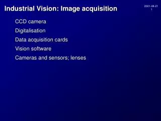
Image Acquisition. Electromagnetic Spectrum. The wavelength required to “see” an object must be the same size of smaller than the object. Image Sensors. Sensor Strips. An Example of Digital Image Acquisition Process. Digital Image Generation. Image Sampling and Quantization.


Image Acquisition
E N D
Presentation Transcript
Electromagnetic Spectrum The wavelength required to “see” an object must be the same size of smaller than the object
An image is a function defined on a 2D coordinate f(x,y). The value of f(x,y) is the intensity. 3 such functions can be defined for a color image, each represents one color component A digital image can be represented as a matrix. Digital Image Representation
Spatial resolution: # of samples per unit length or area DPI: dots per inch specifies the size of an individual pixel If pixel size is kept constant, the size of an image will affect spatial resolution Gray level resolution: Number of bits per pixel Usually 8 bits Color image has 3 image planes to yield 8 x 3 = 24 bits/pixel Too few levels may cause false contour Spatial and Gray Level Resolution
Size, Quantization Levels and Details Isopreference curves
A band-limited continuous signal can be reconstructed perfectly from its discrete-time samples if the sampling rate is above the Nyquist rate Frequency domain interpretation: Sampling Theory BL continuous time signal f Sampled discrete time signal f reconstructed cont. time signal f
xc(t): Band-limited continuous time signal X() = 0 for | | o, X(): Fourier spectrum Sampled at t = nT where T: sampling period, and fs = 1/T: sampling frequency x(n) = xc(nT) has spectrum Note that X() = X(T) is a periodic extension of X() To reconstruct, convolve with inverse Fourier transform of an ideal low pass filter, leading to a sinc function in spatial domain. Often approximate the sinc function by pulse (sample and hold circuit), followed by a low pass filter. Sampling Theory Derivation