Challenges in Mobile Communication Modulation Techniques
Explore modulation techniques in mobile communications, including fading, energy efficiency, digital modulation, and channel bandwidth. Learn about linear and non-linear modulation, such as amplitude and phase modulations like BPSK, QPSK, and GMSK.


Challenges in Mobile Communication Modulation Techniques
E N D
Presentation Transcript
Modulation Techniques Dr. J. Martin Leo Manickam Professor
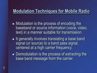
Challenges in Mobile Communication • Channel • fading • Energy • Bandwidth
Digital Modulation • Digital signal is converted into analog bit stream
Classification Linear modulation Non linear (constant envelope) modulation Amplitude of the transmitted signal does not vary with the amplitude of the message signal Power efficient class C amplifiers can be used Low out of band radiation Limiter-discriminator can be used for demodulation FSK,MSK, GMSK • Amplitude of the transmitted signal varies linearly with message signal • Bandwidth efficient • QPSK, OQPSK
BPSK BPSK is equivalent to a DSB/SC
Minimum Shift Keying (MSK) • Phase information is used to improve the noise performance of the receiver • CPFSK signal (0≤t ≤Tb) • Eb – transmitted signal energy • Tb – Bit duration • Θ(0) – value of the phase at t=0, sums up the past history of the modulation process upto t=0.
Phase tree • At time t =Tb,
Signal space diagram Quadrature component will be half cycle sine wave In-phase component will be half cycle cosine wave + sign corresponds to - sign corresponds to + sign corresponds to - sign corresponds to
As and can each assume two possible values, any one of four possible values can arise • Orthonormal basis functions
The MSK signal can represented by • Where s1 and s2 are related to the phase states and , respectively. • Evaluating s1 and s2:
Observation • Both integrals are evaluated for a time interval equal to twice the bit duration • Both lower and upper limits of the product integration used to evaluate s1 are shifted by Tb w.r.t those used to evaluate the s2. • The time interval , for which the phase states and are defined are common to both intervals • Signal space of MSK is two dimensional with four message points
Optimum detection of • If x1 > 0, receiver choose the estimate • If x1 < 0, receiver choose the estimate • Optimum detection of • if x2 > 0, receiver choose the estimate • If x2 < 0, receiver choose the estimate
Symbol – 0 Symbol – 1 Probability of error Same as that of the BPSK and QPSK Estimates
PSD of MSK • MSK has lower sidelobes than QPSK and OQPSK • Faster roll off • Less spectrally efficient • Main lobe of MSK is wider • Bandlimiting is easier • Continuous phase • Amplified using non linear amplifiers • Constant phase • Simple modulation and demodulation
GMSK output NRZ data Gaussian LPF FM Transmitter GMSK modulation • Sidelobe levels of the spectrum are further reduced • Pulse shaping filter requirements • Narrow bandwidth • Sharp cutoff frequencies • Low overshoot • Carrier phase must be ±π/2 at odd multiples and two values 0 and π at even multiples
Impulse response • Transfer function • parameter related to B, the 3dB baseband bandwidth by • GMSK filter may be completely specified by B and the basedand symbol duration T
PSD of a GMSK signal • When BT = ∞, GMSK is equivalent to MSK • When BT decreases, sidelobe levels falls off rapidly • At BT = 0.5, peak of the sidelobe level is 30 db and 20 db below the main lobe for GMSK and MSK • Reducing BT increases the error rate produced by the LPF due to ISI
Table 6.3 Occupied RF bandwidth (for GMSK and MSK as a fraction of Rb). Containing the given percentage of power • GMSK is spectrally tighter than MSK • GMSK spectrum is compact at smaller values of BT but degradation due to ISI increases.
is a constant related to BT by GMSK Bit error rate
Combined Linear and Constant Envelope Modulation Techniques • Varying envelope and phase (or frequency) of an RF carrier (M-ary modulation) • Two or more bits are grouped together to form symbols and one of M possible symbols are is transmitted during each symbol period • Bandwidth efficient • Power inefficient • Poor error performance (closely located message points
M - ary Phase Shift Keying (MPSK) • Carrier phase takes on one of M possible values • Where Es is the energy per symbol = (log2M)Eb Ts is the symbol period = (log2M)Tb • In quadrature form • Orthonormal basis function:
M – ary PSK can be expressed as • Signal space is 2D and the M-ary message points are equally spaced on a circle of radius at the origin • Distance between the adjacent symbols is equal to • Average symbol error prob. • Q function defined as 8 - PSK
Bandwidth and power efficiency of M-ary PSK signals B: First null bandwidth of M-ary PSK signals
M-ary PSK PSD, for M = 8,16(PSD for both rectangular and RCF pulses for fixed Rb • When M increases (fixed Rb) • First null bandwidth decreases • Bandwidth efficiency increases • Constellation is densely packed • Power efficiency decreases • More sensitive to the timing jitter
M-ary Quadrature amplitude modulation (QAM) • Amplitude and phase of the transmitted signal are varied Where Emin - energy of the signal with the lowest amplitude and ai and bi are a pair of independent integers chosen according to the location of the particular point • No constant energy per symbol • No constant distance between possible symbol states • Si(t) is detected with higher probability than others
Ortho normal basis functions • Coordinates of ith message point: • Where is an element of L by L matrix given by • Where
Constellation Diagram for 16-QAM: • LXL matrix is given by • Probability of Error:
Bandwidth and Power efficiency of QAM • Power spectrum and bandwidth efficiency of QAM is identical to M-ary PSK • Power efficiency is superior than M-ary PSK
M-ary Frequency Shift Keying (MFSK) • Transmitted signal Where for some fixed integer nc • Transmitted signals Si(t) themselves can be used as a complete ortho normal basis functions • M-dimensional signal space, minimum distance is
Average probability of symbol error: Coherent detection: Non coherent detection: • Channel Bandwidth: Coherent MFSK: Non Coherent MFSK:
Bandwidth and Power Efficiency of Coherent MFSK • Can be amplified by using non-linear amplifiers with no performance degradation • When M increases, • bandwidth efficiency decreases • Power efficiency increases
Performance of Digital modulation in Slow Flat-fading channels • Multiplicative gain variation • Received signal can be expressed as - channel gain - phase shift of the channel n(t) - is the additive gaussian noise • Assumptions • Attenuation and phase shift remains constant
Probability of Error in slow flat-fading channel • Choose the possible range for signal strength due to fading • Average the probability of error of the particular modulation in AWGN channel over possible range of signal strength • - Probability of error for an arbitrary modulation at a specific value of SNR X, • - pdf of X due to the fading channel • Eb and No are the average energy per bit and noise PSD in a non-fading AWGN channel • - instantaneous power values of the fading channel, w.r.t the non fading
For rayleigh fading channels ,fading amplitude has rayleigh distribution is the average value of the signal to noise ratio
For large values of Eb/N0: • For GMSK