Download
1 / 19
190 likes | 409 Vues
Modelling the Broad Line Region. Andrea Ruff Rachel Webster University of Melbourne. Outline. The primary goal is to model the geometry, dynamics and physical conditions of the BLR What do we know about the BLR Line ratios, stratification of ionisation Modelling with Cloudy

E N D
Modelling the Broad Line Region Andrea Ruff Rachel Webster University of Melbourne
Outline • The primary goal is to model the geometry, dynamics and physical conditions of the BLR • What do we know about the BLR • Line ratios, stratification of ionisation • Modelling with Cloudy • A simple cloud distribution • Simulations over large parameter space • Further Work
Structure of Quasars • The region is too small to be spatially resolved with a telescope • Peak Quasar population z~2 (~10 billion yrs ago) • What is the BLR? • Regions with no BLR gas, but what are the angles?
Lyα CIV CIII] Quasar spectrum NV
About the BLR • Photo-ionised gas (T from line ratios) • Non-thermal broadening • The gas is moving with a high velocity • Up to 0.1c • Variations in BL fluxes in response to the continuum (point like) • Gas is close to the central BH, but also distributed over a large radius
Broad Emission Line flux ratios • Quasars vary in Luminosity by up to 4 dex • The same emission lines are seen • In the same approximate ratios • Why? • T(photo-ionisation equilibrium) ~ 104K? • Peterson, 2006 • Unlikely, not reflected in simulations • Something else is causing this
Fluxes and time delays Line Relative Emission Time Delay (lt days) Lyα 1216Å 1.00 2 C IV 1549Å 0.4-0.6 10 C III] 1900Å 0.15-0.3 20 Mg II 2798Å 0.15-0.3 44 Data from: Baldwin et al. (1989), Peterson, Francis et al. (1991) for Seyferts
Dynamics of the BLR • Keplarian rotation about the central BH • Assumes gas is from the accretion disk • FWHM is larger for higher E ionisation lines • An outflow has also been suggested by asymmetries in BL profiles • Line separations support this • MHD on small scales • Radiative driving (continuum and line)
Consequences of an Outflow • The optical depth will be modified • Castor (1974) • The optical depth depends on the velocity gradient • This changes not only the emitted flux, but also the shape of emission lines • The rotation will also influence the line profile
Modelling the BLR • Numerical simulation • Cloudy, Gary Ferland and associates • “Spectral simulations for the discriminating astrophysicist since 1978” • Emission is calculated from a set of initial conditions • Gas density, distance from source, source brightness and shape, metallicity, NH, velocity
A Simple Outflow • Using mass conservation: • This gives a power law: • Simulations show that The power law index is way more important than specific cloud conditions
Arbitrary power law Ncαrβ Line density (cm-3) β=1 β=2 β=3 C IV 1549 nH=109 0.451 0.330 0.144 nH=1010 0.518 0.243 .0422 nH=1011 0.760 0.244 .0205 Mg II 2798 nH=109 .0907 0.210 0.293 nH=1010 0.115 0.327 0.448 nH=1011 0.117 0.432 0.614
Parameter Space: EW • EW: reprocessing efficiency • How efficiently the line is produced from the continuum radiation (at 1216Å) • Can get line luminosity from appropriate integration: • Baldwin et al. (1995) • Where f(r) and g(n) are cloud covering fractions • Also gives emission response as a fn of r
These plots show the reprocessing efficiency 3,249 different BLR configurations CIV collisionally excited Also give emission response as a function of r Integration gives line flux The terms in the integration need to be determined using hydrodynamics r2 density
The integration will also give emission as a function of radius Constant density model nH = 1010 cm-3 The chosen hydrogen density will influence this if there is a radial dependence on velocity 2 lt days 10 lt days 44 lt days
Accuracy of a single density model • Further complexity is required • LOC model (Baldwin et al. 1995) • Argues that there is a conglomeration of many different density clouds • Given the distance scales of the BLR, would nH α r-γbe expected? • This dependence should be considered
Summary • The gas distribution is important in calculating emission line ratios • The reason for consistent ratios over 4 orders of luminosity has been established • Using Cloudy: • Simulate relative line intensities • Radius of emission • This model requires a good description of the flow
Further Work • Further investigation of free parameters • Incident continuum, metallicity, turbulence, velocity • Need to make a model! • This model will give line ratios, line shapes, timing predictions
Thanks • Questions?

![[PDF READ ONLINE] Modelling the Midland Region from 1948](https://cdn7.slideserve.com/12360005/slide1-dt.jpg)