Statistical Inference in Management - Homework on Distributions and Z-Scores
500 likes | 604 Vues
Explore creating distributions, z-scores, and connecting probability in statistical inference. Study guide based on Lind and Plous books. Focus on Chapters 5-11. Learn about normal distribution, standard deviation, and probability.

Statistical Inference in Management - Homework on Distributions and Z-Scores
E N D
Presentation Transcript
MGMT 276: Statistical Inference in ManagementFall, 2013 Welcome
Homework due – Thursday (October 10th) On class website: Please complete homework worksheet #9 Creating distributions and tying together with z scores and probability
Please read before our next exam (October 24th) - Chapters 5 - 11 in Lind book - Chapters 10, 11, 12 & 14 in Plous book: Lind Chapter 5: Survey of Probability Concepts Chapter 6: Discrete Probability Distributions Chapter 7: Continuous Probability Distributions Chapter 8: Sampling Methods and CLT Chapter 9: Estimation and Confidence Interval Chapter 10: One sample Tests of Hypothesis Chapter 11: Two sample Tests of Hypothesis Plous Chapter 10: The Representativeness Heuristic Chapter 11: The Availability Heuristic Chapter 12: Probability and Risk Chapter 14: The Perception of Randomness We’ll be jumping around some…we will start with chapter 7
Use this as your study guide By the end of lecture today10/8/13 Measures of variability Standard deviation and Variance Counting ‘standard deviationses’ – z scores Connecting raw scores, z scores and probabilityConnecting probability, proportion and area of curve Percentiles
Mean = 100 Standard deviation = 5 If we go up one standard deviation z score = +1.0 and raw score = 105 If we go down one standard deviation z score = -1.0 and raw score = 95 85 90 95 100 105 110 115 If we go up two standard deviations z score = +2.0 and raw score = 110 If we go down two standard deviations z score = -2.0 and raw score = 90 85 90 95 100 105 110 115 If we go up three standard deviations z score = +3.0 and raw score = 115 If we go down three standard deviations z score = -3.0 and raw score = 85 85 90 95 100 105 110 115 z score: A score that indicates how many standard deviations an observation is above or below the mean of the distribution z score = raw score - mean standard deviation
Raw scores, z scores & probabilities • Notice: • 3 types of numbers • raw scores • z scores • probabilities z = -2 z = +2 Mean = 50 S = 10 (Note S = standard deviation) If we go up two standard deviations z score = +2.0 and raw score = 70 If we go down two standard deviations z score = -2.0 and raw score = 30
z = -1 z = 1 Normal distribution -3 -2 -1 0 +1 +2 +3 z scores -3 -2 -1 0 +1 +2 +3 z scores raw scores In z-score distribution mean = 0 standard deviation = 1 In a normal distribution mean = µstandard deviation = σ
Characteristics of Normal Distribution We’re talking about distribution of raw scores Normal Distribution How would you describe the shape? Symmetric and bell-shaped Shape
Characteristics of Normal Distribution Normal Distribution What is the standard deviation? σ Standard Deviation Shape Symmetric and bell-shaped
Characteristics of Normal Distribution Normal Distribution What is the mean? µ Mean Standard Deviationσ Shape Symmetric and bell-shaped
Characteristics of Normal Distribution Normal Distribution What is the theoretical range? -∞< X < +∞ Domain Mean µ Standard Deviationσ Shape Symmetric and bell-shaped
Characteristics of Normal Distribution What is the ‘practical’ range(covers 99.7% of curve) Normal Distribution µ - 3σ< X < µ + 3σ -∞< X < +∞ Domain Mean µ Standard Deviationσ Shape Symmetric and bell-shaped
Characteristics of Normal Distribution Once we know the mean (anchor point) and standard deviation (spread) we can define any normal curve Normal Distribution Parameters µ = population σ= population standard deviation -∞< X < +∞ Domain Mean µ Standard Deviationσ Shape Symmetric and bell-shaped
Characteristics of Normal Distribution Normal Distribution Parameters µ = population σ= population standard deviation -∞< X < +∞ Domain Mean µ Standard Deviationσ Shape Symmetric and bell-shaped
Characteristics of Standard Normal Distribution (distribution of z-scores) Normal Distribution How would you describe the shape? Shape Symmetric and bell-shaped
Characteristics of Standard Normal Distribution (curve of z-scores) Normal Distribution The standard deviation in a z-distribution is always 1 (when you go up one standard deviation go up one z score) Standard Deviation 1 Shape Symmetric and bell-shaped
Characteristics of Standard Normal Distribution (curve of z-scores) Normal Distribution What z-score is associated with the mean of the distribution? Mean 0 Standard Deviation1 Shape Symmetric and bell-shaped
Characteristics of Standard Normal Distribution Normal Distribution What is the theoretical range? -∞< Z < +∞ Domain Mean 0 Standard Deviation1 Shape Symmetric and bell-shaped
Characteristics of Standard Normal Distribution Normal Distribution Parameters µ = population σ= population standard deviation -∞< Z < +∞ Domain Mean 0 Standard Deviation1 Shape Symmetric and bell-shaped
Characteristics of Standard Normal Distribution (curve of z-scores) Normal Distribution Parameters µ = population σ= population standard deviation -∞< Z < +∞ Domain Mean 0 Standard Deviation1 Shape Symmetric and bell-shaped
z = -1 z = 1 Normal distribution -3 -2 -1 0 +1 +2 +3 z scores -3 -2 -1 0 +1 +2 +3 z scores raw scores In z-score distribution mean = 0 standard deviation = 1 In a normal distribution mean = µstandard deviation = σ
. Homework Worksheet
. Homework Worksheet: Problem 1 1 sd 1 sd .68 30 32 28
. Homework Worksheet: Problem 2 2 sd 2 sd .95 32 28 34 26 30
. Homework Worksheet: Problem 3 3 sd 3 sd .997 24 36 32 28 34 26 30
. Homework Worksheet: Problem 4 .50 24 36 32 28 34 26 30
. Homework Worksheet: Problem 5 Go to table 33-30 z = 1.5 z = .4332 2 .4332 24 36 32 28 34 26 30
. Homework Worksheet: Problem 6 Go to table 33-30 z = 1.5 z = .4332 2 .9332 .4332 .5000 24 36 32 28 34 26 30
.0668 Go to table 33-30 .4332 z = 1.5 z = .4332 2 33 .5000 - .4332 = .0668 Go to table 29-30 z =-.5 z = .1915 .5000 .1915 2 .5000 + .1915 = .6915 29 .4938 .1915 25-30 25 31 z = -2.5 z = .4938 2 .4938 + .1915 = .6853 Go to table 31-30 z =.5 z = .1915 2 .0668 .4332 27-30 z = -1.5 z = .4332 27 .5000 - .4332 = .0668 2
Problem 11: .5000 + .4938 = .9938 Problem 12: .5000 - .3413 = .1587 Problem 13: 30 Problem 14: 28 and 32
. 77th percentile Go to table nearest z = .74 .2700 x = mean + z σ = 30 + (.74)(2) = 31.48 .7700 .27 .5000 24 36 ? 28 34 26 30 31.48
. 13th percentile Go to table nearest z = 1.13 .3700 x = mean + z σ = 30 + (-1.13)(2) = 27.74 .37 .50 .13 ? 24 36 32 27.74 34 26 30
Problem 17: 68% or .68 or 68.26% or .6826 Problem 18: 95% or .95 or 95.44% or .9544 Problem 19: 99.70% or .9970 Problem 20: 27.34% or .2734 Problem 21: 40.13% or .4013 Problem 22: 69.15% or .6915 Problem 23: 18.41% or .1841 Problem 24: 28.81% or .2881 Problem 25: 96.93% or .9693 or 96.93% or .9693 Problem 26: .89% or .0089 Problem 27: 95.99% or .9599 Problem 28: 4.01% or .0401 Problem 29: 293.2 x = mean + z σ = 200 + (2.33)(40) = 293.2 Problem 30: 182.4 x = mean + z σ = 200 + (-.44)(40) = 182.4 Problem 31: 190 Problem 32: 217.6
. Find score associated with the 75th percentile 75th percentile Go to table nearest z = .67 .2500 x = mean + z σ = 30 + (.67)(2) = 31.34 .7500 .25 .5000 24 36 ? 28 34 26 30 31.34 z = .67
. Find the score associated with the 25th percentile 25th percentile Go to table nearest z = -.67 .2500 x = mean + z σ = 30 + (-.67)(2) = 28.66 .2500 .25 .25 28.66 24 ? 36 28 34 26 30 z = -.67
Variability and means Variability and means 38 40 44 48 52 56 58 The variability is different…. The mean is the same … What might the standard deviation be? 38 40 44 48 52 56 58 Remember to keep number lines same for both examples
Variability and means Grades of all students in the class • 65 70 75 80 85 90 • Grades Grades of “C” students What might the standard deviation be? What might this be an example of? • 65 70 75 80 85 90 • Grades Other examples?
Variability and means Remember, there is an implied axis measuring frequency f 60 65 70 75 80 85 90 f Remember to keep number lines equally spaced 60 65 70 75 80 85 90 Remember to keep number lines same for both examples Variable must be numeric
Variability and means Birth weight for infants From entire population 1 3 5 7 9 11 13 Birth weight in pounds Birth weight for infants from a “typical family” What might the standard deviation be? What might this be an example of? • 3 5 7 9 11 13 • Birth weight in pounds Other examples? Notice: number lines equally spaced
Variability and means Social distance norm(personal space) for international community 40 50 60 70 80 90 100Social Distance Norm Social distance norm (personal space) for Tucson What might the standard deviation be? What might this be an example of? 40 50 60 70 80 90 100 Social Distance Norm Other examples? Notice: number lines equally spaced
Variability and means Distributions same mean different variability Final exam scores “C” students versus whole class Birth weight within a typical family versus within the whole community Running speed 30 year olds vs. 20 – 40 year olds Number of violent crimes Milwaukee vs. whole Midwest Social distance (personal space) California vs international community
Variability and means Distributions different mean same variability Performance on a final exam Before versus after taking the class 40 50 60 70 80 90 100 Score on final (before taking class) 40 50 60 70 80 90 100 Score on final (before taking class) Notice: number lines equally spaced
Variability and means Distributions different mean same variability Height of men versus women 62 64 66 68 70 72 74 76Inches in height (women) 62 64 66 68 70 72 74 76Inches in height (men) Notice: number lines equally spaced
Variability and means Distributions different mean same variability Driving ability Talking on a cell phone or not 2 4 6 8 10 12 14 16Number of errors (not on phone) 2 4 6 8 10 12 14 16Number of errors (on phone) Notice: number lines equally spaced
Variability and means Comparing distributions different mean same variability Performance on a final exam Before versus after taking the class Height of men versus women Driving ability Talking on a cell phone or not Notice: number lines equally spaced
. Writing Assignment (also Homework #9)Comparing distributions (mean and variability) • Think of examples for these three situations • same mean but different variability • same variability but different means • same mean and same variability (different groups) • estimate standard deviation • calculate variance • for each curve find the raw score for the z’s given Remember: number lines equally spaced
Hand in homework & worksheet
Thank you! See you next time!!