Instruction-Level Parallelism compiler techniques and branch prediction

1. Instruction-Level Parallelismcompiler techniques and branch prediction prepared and Instructed by Shmuel Wimer Eng. Faculty, Bar-Ilan University Instruction-Level Parallelism 1

2. Concepts and Challenges The potential overlap among instructions is called instruction-level parallelism (ILP). • Two approaches exploiting ILP: • Hardware discovers and exploit the parallelism dynamically. • Software finds parallelism, statically at compile time. • CPI for a pipelined processor: • Ideal pipeline CPI + Structural stalls + Data hazard stalls + Control stalls • Basic block:a straight-line code with no branches. • Between three to six instructions typical size . • Too small to exploit significant amount of parallelism. • We must exploit ILP across multiple basic blocks. Instruction-Level Parallelism 1

3. Instruction-Level Parallelism 1

4. Loop-level parallelism exploits parallelism among iterations of a loop. A completely parallel loop adding two 1000-element arrays: Within an iteration there is no opportunity for overlap, but every iteration can overlap with any other iteration. The loop can be unrolled either statically by compiler or dynamically by hardware. Vector processing is also possible. Supported in DSP, graphics, and multimedia applications. Instruction-Level Parallelism 1

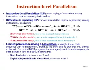
5. Data Dependences and Hazards If two instructions are parallel, they can be executed simultaneously in a pipeline without causing any stalls, assuming the pipeline has sufficient resources. Two dependent instructions must be executed in order, but can often be partially overlapped. Three types of dependences: data dependences, name dependences, and control dependences. • Instruction jisdata dependent on instruction iif: • iproduces a result that may be used by j, or • jis data dependent on an instruction k, and kis data dependent on i. Instruction-Level Parallelism 1

6. The following loop increments a vector of values in memory starting at 0(R1), with the last element at 8(R2)), by a scalar in register F2. The data dependences in this code sequence involve both floating-point and integer data. Since between two data dependent instructions there is a chain of one or more data hazards, they cannot execute simultaneously or be completely overlapped. Instruction-Level Parallelism 1

7. Data dependence conveys: • the possibility of a hazard, • the order in which results must be calculated, and • an upper bound on how much parallelism can be exploited. • Detecting dependence registers is straightforward. • Register names are fixed in the instructions. • Dependences that flow through memory locations are more difficult to detect. • Two addresses may refer to the same location but look different: For example, 100(R4) and20(R6). • The effective address of a load or store may change from one execution of the instruction to another (so that 20(R4) and20(R4) may be different). Instruction-Level Parallelism 1

8. Name Dependences A name dependence occurs when two instructions use the same register or memory location, called a name, but there is no flow of data between the instructions. If iprecedes jin program order: Anti dependencebetween iand joccurs when jwrites a register or memory location that ireads. The original ordering must be preserved to ensure that ireads the correct value. Instruction-Level Parallelism 1

9. Output dependence occurs when iand jwrite the same register or memory location. Their ordering must be preserved to ensure proper value written by j. • Name dependence is not a true dependence. • The instructions involved can execute simultaneously or be reordered. • The name (register # or memory location) is changed so the instructions do not conflict. • Register renamingcan be more easily done. • Done either statically by a compiler or dynamically by the hardware. Instruction-Level Parallelism 1

10. Data Hazards • A hazard is created whenever a dependence between instructions is close enough. • Program ordermust be preserved. • The goal of both SW and HW techniquesis to exploit parallelism by preserving program order only where it affects the outcome of the program. • Detecting and avoiding hazards ensures that necessary program order is preserved. • Data hazards are classifieddepending on the order of read and write accesses in the instructions. Consider two instructions iandj, withiprecedingj Instruction-Level Parallelism 1

11. The possible data hazards are: • RAW (read after write). jtries to read a source before iwrites it. • The most common, correspondingto a true data dependence. • Program order must be preserved. • WAW (write after write). jtries to write an operand before it is written by i. • Writes are performed in the wrong order, leaving the value written by irather than by j. • Correspondsto an output dependence. • Present only in pipelines that write in more than one pipe stage or allow an instruction to proceed even when a previous instruction is stalled. Instruction-Level Parallelism 1

12. WAR (write after read). jtries to write a destination before it is read by i, so i incorrectly gets the new value. • Arises from an anti dependence. • Cannot occur in most static issue pipelines because all reads are early (in ID) and all writes are late (in WB). • Occurs when there are some instructions that write results early in the pipeline andother instructions that read a source late in the pipeline. • Occurs also when instructions are reordered. Instruction-Level Parallelism 1

13. Control Dependences A control dependence determines the ordering of iwith respect to a branch so that the iis executed in correct order and only when it should be. • There are two constraints imposed by control dependences: • An instruction that is control dependent on a branch cannot be moved before the branch so that its execution is no longer controlled by the branch. • An instruction that is not control dependent on a branch cannot be moved afterthe branch so that its execution is controlled by the branch. Instruction-Level Parallelism 1

14. Consider this code: If we do not maintain the data dependence involving R2, the result of the program can be changed. If we ignore the control dependence and move the load before the branch, the load may cause a memory protection exception. (why?) No data dependence prevents interchanging the BEQZ and the LW; it is only the control dependence. Instruction-Level Parallelism 1

15. Compiler Techniques for Exposing ILP Pipeline is kept full by finding sequences of unrelated instructions that can be overlapped in the pipeline. Toavoid stall, a dependent instruction must be separated from the source by a distance in clock cycles equal to the pipeline latency of that source. Example: Latencies of FP operations Instruction-Level Parallelism 1

16. Code adding scalar to vector: Straightforward MIPS assembly code: R1 is initially the address top element in the array. F2 contains the scalar value s. R2 is pre computed, so that 8(R2) is the array bottom. Instruction-Level Parallelism 1

17. Without any scheduling the loop takes 9 cycles: Scheduling the loop obtains only two stalls, taking 7 cycles: Instruction-Level Parallelism 1

18. The actual work on the array is just 3/7 cycles (load, add, and store). The other 4 are loop overhead. Their elimination requires more operations relative to the overhead. • Loop unrollingreplicatingthe loop body multiple times can be used. • Adjustment of the loop termination code is required. • Used also to improve scheduling. Instruction replication alone with usage of same registers could prevent effective scheduling. Different registers for each replication are required (increasing the required number of registers). Instruction-Level Parallelism 1

19. Unrolled code (not rescheduled) 2 stalls 2 stalls 2 stalls 2 stalls 1 stall 1 stall 1 stall 1 stall 1 stall Stalls are still there. Run in 27 clock cycles, 6.75 per element. Instruction-Level Parallelism 1

20. Unrolled and rescheduled code No stalls required. Execution dropped 14 clock cycles, 3.5 per element. Compared with 9 per element before unrolling or scheduling and 7 when scheduled but not unrolled. Instruction-Level Parallelism 1

21. Problem: The number of loop iterations nis usually unknown. We would like to unroll the loop to make kcopies of its body. Two consecutive loops are generated Instead. Thefirst executes n mod ktimes and has a body that is the original loop. The second is the unrolled body surrounded by an outer loop that iterates n/ktimes. Forlarge n, most of the execution time will be spent in the unrolled loop body. Instruction-Level Parallelism 1

22. Branch Prediction performance losses can be reduced by predicting how branches will behave. Branch prediction (BP) Can be done statically at compilation and dynamically at execution time. The simplest static scheme is to predict a branch as taken. Misprediction equal to the untakenfrequency (34% for the SPEC benchmark). BP based on profiling is more accurate. Instruction-Level Parallelism 1

23. Misprediction on SPEC92 for a profile-based predictor Instruction-Level Parallelism 1

24. Dynamic Branch Prediction The simplest is a BP buffer, a small 1-bit memory indexed by the lower portion of the address of the branch instruction. Useful only to reduce the branch delay when it is longer than the time to compute the possible target PCs. BP mayhave been put there by another branch that has the same low-order address bits! Fetching begins in the predicted direction. If it was wrong, the BP bit is inverted and stored back. Instruction-Level Parallelism 1

25. Problem: Even if almost always taken, We will likely predict incorrectly twice. (Why?) Solution: 2-bit BP are often used. It must miss twice before it is changed. An n-bit counter is possible. If counter > 2n-1– 1, taken is predicted; otherwise, untaken. 2-bit do almost as well, thus used by most systems. Instruction-Level Parallelism 1

26. Correlating Branch Predictors 2-bit uses only the recent behavior of a single branch for BP. Accuracy can be improved if the recent behavior of otherbranches are considered. Consider the code: Let aa and bb be assigned to registers R1 and R2, and label the three branches b1, b2, and b3. The compiler generates the typical MIPS code: Instruction-Level Parallelism 1

27. The behavior of b3 is correlated with that of b1 and b2. A predictor using only the behavior of a single branch to predict its outcome is blind of this behavior. Correlating or two-levelpredictorsadd information about the most recent branches to decide on a branch. Instruction-Level Parallelism 1

28. An (m,n) BP uses the last mbranches to choose from 2m n-bit BPs for a single branch. More accurate than 2-bit and requires simple HW. The global history of the most recent mbranches is recorded in an m-bit shift register.The buffer is indexed using a concatenation of the low-order branch address bitswith the m-bit history. The 6-bit index of a 64 entries (2,2) buffer is formed by the 4 low-order bits of the branch address + 2 global bits obtained from the two most recent branches. Instruction-Level Parallelism 1

29. For a fair comparison of the performance of BPs, the same number of state bits are used. The number of bits in an (m,n) predictor is: 2m× n × # of prediction entries. A 2-bit predictor w/o global history is a (0,2) predictor. Example: How many bits are in the (0,2) BP with 4K entries? How many entries are in a (2,2) predictor with the same number of bits? A 4K-entries BP has 20× 2 × 4K = 8K bits. A (2,2) BP having a total of 8K bits satisfies 22× 2 × # of prediction entries = 8K. The # of prediction entries is therefore = 1K. Instruction-Level Parallelism 1

30. significant improvement not much improvement Instruction-Level Parallelism 1

31. Tournament Predictors Tournament predictors combine predictors based on global and local information. They achieve better accuracy and effectively use very large numbers of prediction bits. Tournament BPs use a 2-bit saturating counter per branch to select between two different BP (local, global), based on which was most effective in recent predictions. As in a simple 2-bit predictor, the saturating counter requires two mispredictions before changing the identity of the preferred BP. Instruction-Level Parallelism 1

32. Instruction-Level Parallelism 1